1 - DIPS Quick Start
1.0 Introduction
DIPS is a program designed for the interactive analysis of orientation-based geological data. The program is capable of various applications and is designed for both novice users and experienced users of stereographic projection who wish to utilize more advanced tools in the analysis of geological data.
DIPS allows the user to analyze and visualize structural data following the same techniques used in manual stereonets.
This tutorial provides a quick tour of the major plotting features of DIPS. A typical example file is used to illustrate Stereonet 2D plots, Stereonet 3D plots, and Rosette plots.
Topics Covered in this Tutorial:
- Project Settings
- Orientation Data
- Pole Data Grid
- Stereonet 2D
- Stereonet 3D
- Rosette
- Vector Plot
- Report Generator
Finished Product:
The finished product of this tutorial can be found in the Tutorial 01 Quick Start.dips9 file, located in the Examples > Tutorials folder in your DIPS installation folder.
2.0 Model
If you have not already done so, run DIPS by double-clicking on the DIPS icon in your installation folder. Or from the Start menu, select Programs > Rocscience > DIPS > DIPS.
If the DIPS application window is not already maximized, maximize it now, so that the full screen is available for viewing the model.
DIPS comes with several example files installed with the program. These example files can be accessed by selecting File > Recent > Examples Folder from the File menu (or File > Open from the Home ribbon). This tutorial will use the Example.dips9 file to demonstrate the basic plotting features of DIPS.
- Select File > Recent > Examples Folder
 from the menu.
 - Open the Example.dips9 file. Since we will be using the Example.dips9 file in other tutorials, save this example file with a new file name without overwriting the original file.
- Select File > Save As
 from the menu.
 - Enter the file name Tutorial 01 Quick Start and Save the file.
3.0 Pole Data Grid
If the Pole Data Grid is not already the active view:
- Select the Pole Data Grid view tab.
You should see the Pole Data Grid view shown in the following figure.
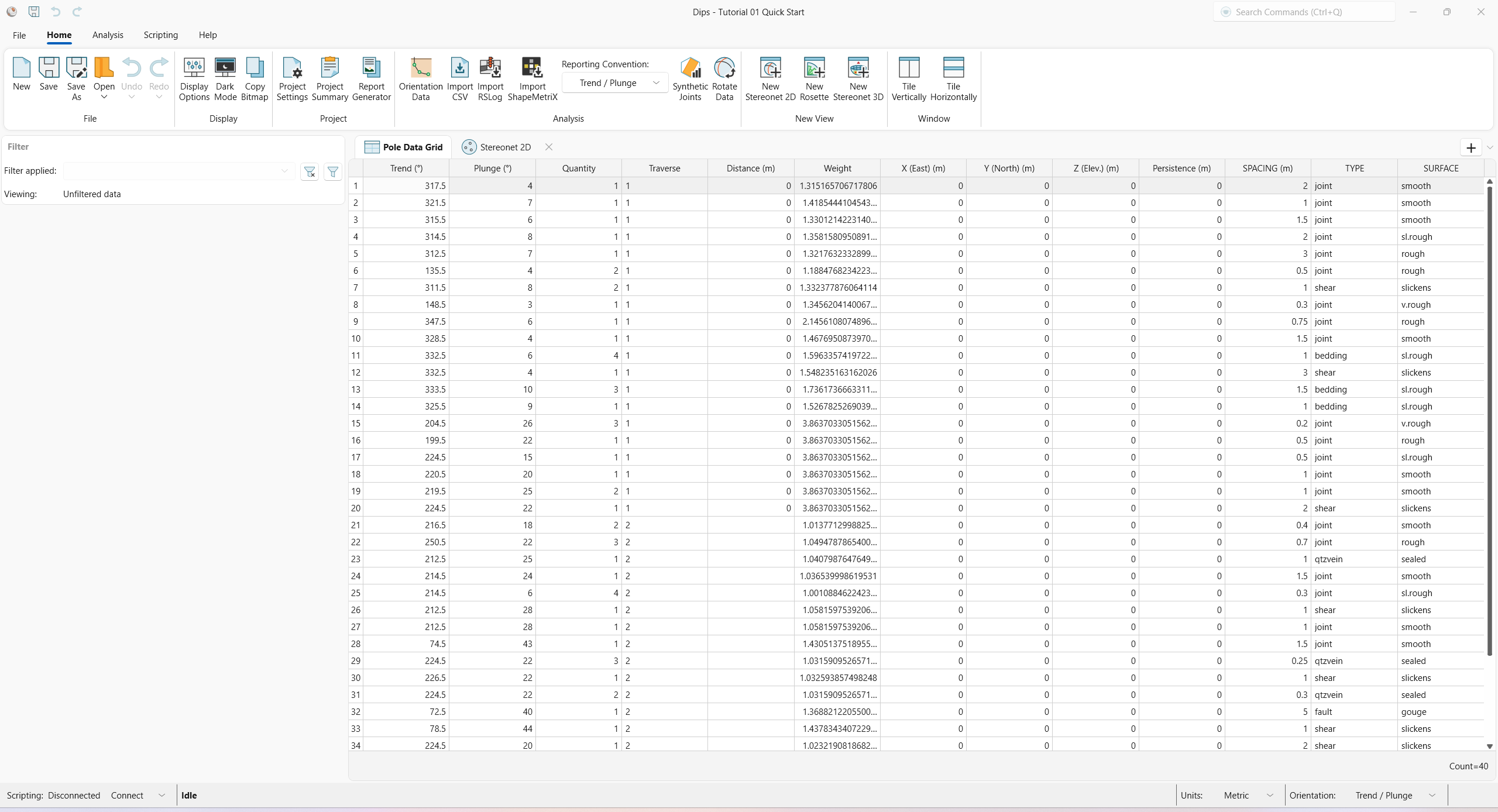
The Pole Data Grid shows all processed orientation data entered in the Orientation Data dialog. Note that there are 40 rows of data (i.e., Count=40) and the following columns:
- Trend and Plunge columns showing the processed orientations in the selected Reporting Orientation.
- Quantity column
- Traverse column
- Distance column
- Weight column
- X (East) column
- Y (North) column
- Z (Elev.) column
- Persistence column
- Three extra columns (i.e., SPACING, TYPE, SURFACE)
3.1 Project Settings
The Project Settings contain options for the Reporting Conventions of Units and Orientation.
- Select Home > Project > Project Settings
 from ribbon. The Project Settings dialog appears.
 - Units = Metric. All units are converted to the equivalent metric units (e.g., Length as m)
- Orientation = Dip / Dip Direction. All planar orientations are converted to the equivalent orientation format.
TIP: Alternatively, Unit and Orientation reporting conventions can be changed in the status bar drop downs at the bottom of the application.
The Orientation reporting convention affects the planar orientation formats in the Pole Data Grid and in dialogs (e.g., Edit User Plane, Edit Set Window). The tracked cursor orientation coordinates reported at the bottom-right of the status bar also correspond to the selected Orientation reporting convention.
3.2 Orientation Data
The Orientation Data dialog is the primary data input for DIPS orientation data. To review the raw, unprocessed input data:
- Select Home > Analysis > Orientation Data
 from the ribbon.
 - The Orientation Data dialog appears.
- Note that there are three datasets (or traverses).
- Select dataset 1.
- The Name = 1 and acts as its unique identifier and is used for traverse associations in the Traverse column of the Pole Data Grid.
- The Type = Linear Scanline. See the Traverse Types topic for more information.
- In the Traverse tab:
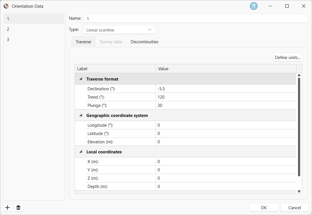
Dataset 1 Traverse tab in the Orientation Data dialog - Declination = -5.5 degrees. See the Declination topic for more information.
- Trend = 120 degrees.
- Plunge = 30 degrees. See the Traverse and Traverse Format topics for more information.
- Comment = Level 3,Stope 3.A,sublevel 310.
- In the Discontinuities tab:
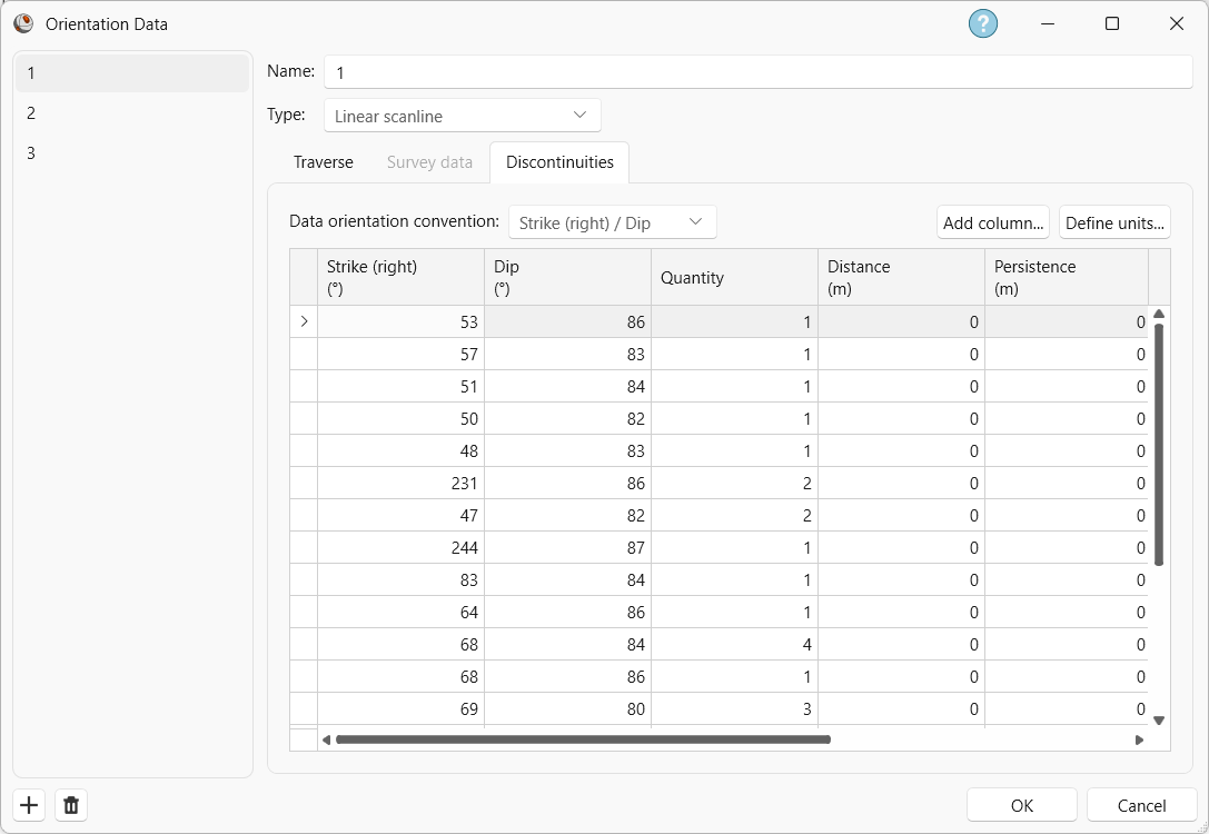
Dataset 1 Discontinuities tab in the Orientation Data dialog - Data Orientation Convention = Strike (right) / Dip. This dictates the orientation format of the first two columns.
- There are 20 rows of discontinuity data:
Strike (right) (°) |
Dip (°) |
Quantity |
X (East) (m) |
Y (North) (m) |
Z (Elev.) (m) |
Persistence (m) |
SPACING (m) |
TYPE |
SURFACE |
53 |
86 |
1 |
0 |
0 |
2 |
joint |
smooth |
53 |
86 |
57 |
83 |
1 |
0 |
0 |
1 |
joint |
smooth |
57 |
83 |
51 |
84 |
1 |
0 |
0 |
1.5 |
joint |
smooth |
51 |
84 |
50 |
82 |
1 |
0 |
0 |
2 |
joint |
sl.rough |
50 |
82 |
48 |
83 |
1 |
0 |
0 |
3 |
joint |
rough |
48 |
83 |
231 |
86 |
2 |
0 |
0 |
0.5 |
joint |
rough |
231 |
86 |
47 |
82 |
2 |
0 |
0 |
1 |
shear |
slickens |
47 |
82 |
244 |
87 |
1 |
0 |
0 |
0.3 |
joint |
v.rough |
244 |
87 |
83 |
84 |
1 |
0 |
0 |
0.75 |
joint |
rough |
83 |
84 |
64 |
86 |
1 |
0 |
0 |
1.5 |
joint |
smooth |
64 |
86 |
68 |
84 |
4 |
0 |
0 |
1 |
bedding |
sl.rough |
68 |
84 |
68 |
86 |
1 |
0 |
0 |
3 |
shear |
slickens |
68 |
86 |
69 |
80 |
3 |
0 |
0 |
1.5 |
bedding |
sl.rough |
69 |
80 |
61 |
81 |
1 |
0 |
0 |
1 |
bedding |
sl.rough |
61 |
81 |
300 |
64 |
3 |
0 |
0 |
0.2 |
joint |
v.rough |
300 |
64 |
295 |
68 |
1 |
0 |
0 |
0.5 |
joint |
rough |
295 |
68 |
320 |
75 |
1 |
0 |
0 |
0.5 |
joint |
sl.rough |
320 |
75 |
316 |
70 |
1 |
0 |
0 |
1 |
joint |
smooth |
316 |
70 |
315 |
65 |
2 |
0 |
0 |
1 |
joint |
smooth |
315 |
65 |
320 |
68 |
1 |
0 |
0 |
2 |
shear |
slickens |
320 |
68 |
- The three extra columns (SPACING, TYPE, and SURFACE) were added using the Add Column button. Note that the SPACING column has units of Length in m. The units can be set when adding a column and are editable by clicking the Define Units button. See the Discontinuities and Units topics for more information.
- Select dataset 2.
- The Name = 2.
- The Type = Planar Mapping. See the Traverse Types topic for more information.
- In the Traverse tab:
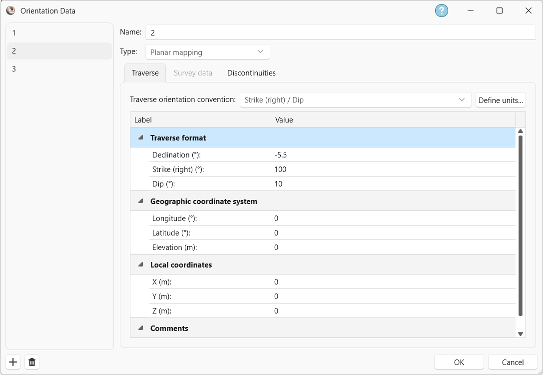
Dataset 2 Traverse tab in the Orientation Data dialog - Traverse Orientation Convention = Strike (right) / Dip.
- Declination = -5.5 degrees.
- Strike (right) = 100 degrees.
- Dip = 10 degrees.
- Comment = Level 5,Stope 5.D roof before shrinkage.
- In the Discontinuities tab:
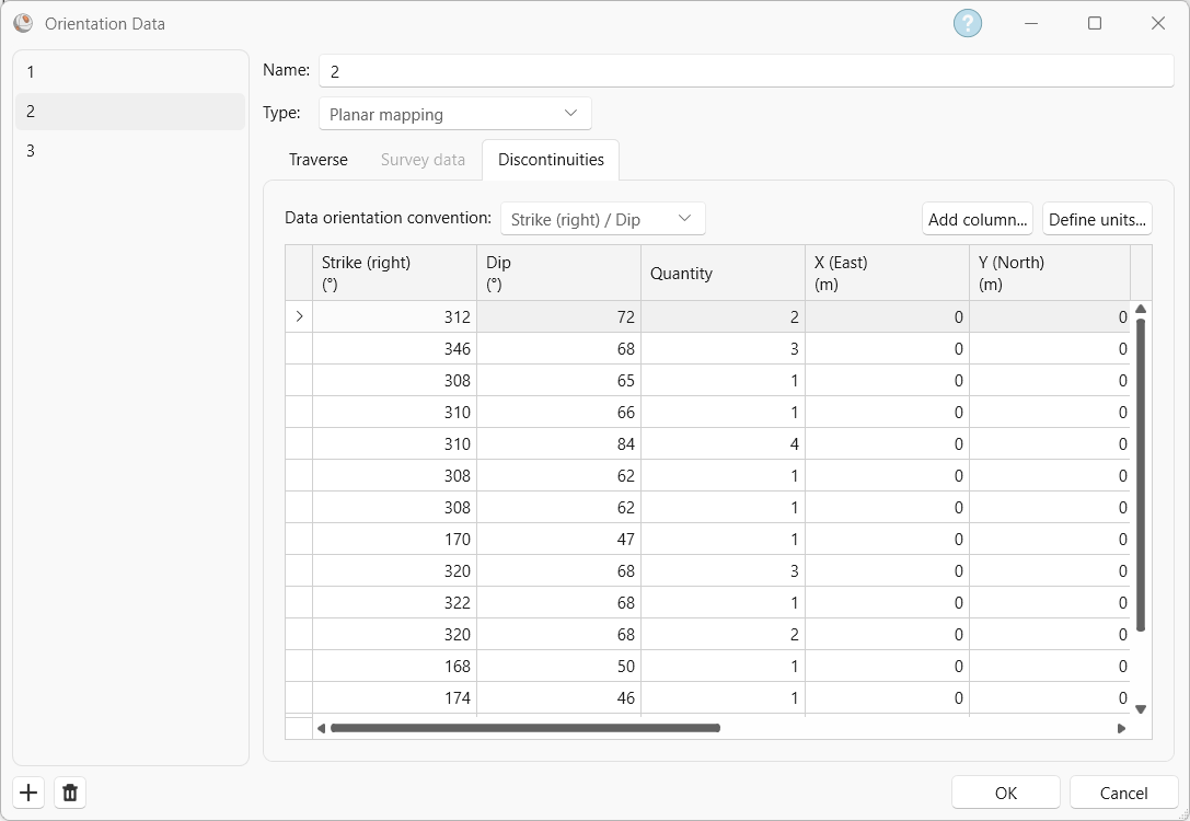
Dataset 2 Discontinuities tab in the Orientation Data dialog - Data Orientation Convention = Strike (right) / Dip. This dictates the orientation format of the first two columns.
- There are 15 rows of discontinuity data:
Strike (right) (°) |
Dip (°) |
Quantity |
X (East) (m) |
Y (North) (m) |
Z (Elev.) (m) |
Persistence (m) |
SPACING (m) |
TYPE |
SURFACE |
312 |
72 |
2 |
0 |
0 |
0 |
0 |
0.4 |
joint |
smooth |
346 |
68 |
3 |
0 |
0 |
0 |
0 |
0.7 |
joint |
rough |
308 |
65 |
1 |
0 |
0 |
0 |
0 |
1 |
qtzvein |
sealed |
310 |
66 |
1 |
0 |
0 |
0 |
0 |
1.5 |
joint |
smooth |
310 |
84 |
4 |
0 |
0 |
0 |
0 |
0.3 |
joint |
sl.rough |
308 |
62 |
1 |
0 |
0 |
0 |
0 |
1 |
shear |
slickens |
308 |
62 |
1 |
0 |
0 |
0 |
0 |
1 |
joint |
smooth |
170 |
47 |
1 |
0 |
0 |
0 |
0 |
1.5 |
joint |
smooth |
320 |
68 |
3 |
0 |
0 |
0 |
0 |
0.25 |
qtzvein |
sealed |
322 |
68 |
1 |
0 |
0 |
0 |
0 |
1 |
shear |
slickens |
320 |
68 |
2 |
0 |
0 |
0 |
0 |
0.3 |
qtzvein |
sealed |
168 |
50 |
1 |
0 |
0 |
0 |
0 |
5 |
fault |
gouge |
174 |
46 |
1 |
0 |
0 |
0 |
0 |
1 |
shear |
slickens |
320 |
70 |
1 |
0 |
0 |
0 |
0 |
2 |
shear |
slickens |
170 |
50 |
1 |
0 |
0 |
0 |
0 |
3 |
joint |
smooth |
- The three extra columns (SPACING, TYPE, and SURFACE) were added using the Add Column button. The extra columns have matching Column Names and Data Type with dataset 1’s Discontinuities extra columns. The Column Name is a unique identifier that allows matching columns to be compiled under a single column in the Pole Data Grid. For any columns with matching Column Name, the Data Type must also match (i.e., it must represent the same type of data), but can have mixed Formats (i.e., Length can be m or ft).
- Select dataset 3.
- The Name = 3.
- The Type = Planar Mapping.
- In the Traverse tab:
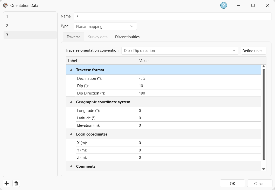
Dataset 3 Traverse tab in the Orientation Data dialog - Traverse Orientation Convention = Dip / Dip Direction.
- Declination = -5.5 degrees.
- Dip = 10 degrees.
- Dip Direction = 190 degrees.
- Comment = Level 5 Stope 5.D roof(aux data).
- In the Discontinuities tab:
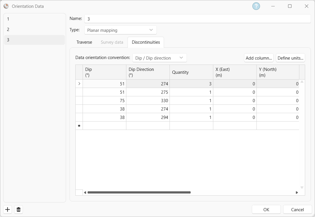
Dataset 3 Discontinuities tab in the Orientation Data dialog - Data Orientation Convention = Dip/Dip Direction. This dictates the orientation format of the first two columns.
- There are 5 rows of discontinuity data:
Dip (°) |
Dip Direction (°) |
Quantity |
X (East) (m) |
Y (North) (m) |
Z (Elev.) (m) |
Persistence (m) |
SPACING (m) |
TYPE |
SURFACE |
51 |
274 |
3 |
0 |
0 |
0 |
0 |
0.3 |
joint |
rough |
51 |
275 |
1 |
0 |
0 |
0 |
0 |
1 |
joint |
rough |
75 |
330 |
1 |
0 |
0 |
0 |
0 |
5 |
fault |
gouge |
38 |
274 |
1 |
0 |
0 |
0 |
0 |
1 |
joint |
sl.rough |
38 |
294 |
1 |
0 |
0 |
0 |
0 |
2 |
joint |
smooth |
51 |
274 |
3 |
0 |
0 |
0 |
0 |
0.3 |
joint |
rough |
51 |
275 |
1 |
0 |
0 |
0 |
0 |
1 |
joint |
rough |
75 |
330 |
1 |
0 |
0 |
0 |
0 |
5 |
fault |
gouge |
- The three extra columns (SPACING, TYPE, and SURFACE) were added using the Add Column button. The extra columns have matching Column Names and Data Type with dataset 1 and 2’s Discontinuities extra columns. The Column Name is a unique identifier that allows matching columns to be compiled under a single column in the Pole Data Grid. For any columns with matching Column Name, the Data Type must also match (i.e., it must represent the same type of data), but can have mixed Formats (i.e., Length can be m or ft).
See the Orientation Data topic for more information.
4.0 Stereonet 2D
Now look at the Stereonet 2D view:
- Select the Stereonet 2D
 view tab.
You should see the Stereonet 2D view shown in the following figure.
4.1.1 Visibility and Properties Panes
When you are viewing a Stereonet 2D view, the Visibility pane on the left side of the application allows you to fully customize the visibility of entities in the stereonet. By selecting the Visibility icon, you can toggle on and off the visibility of individual entities.
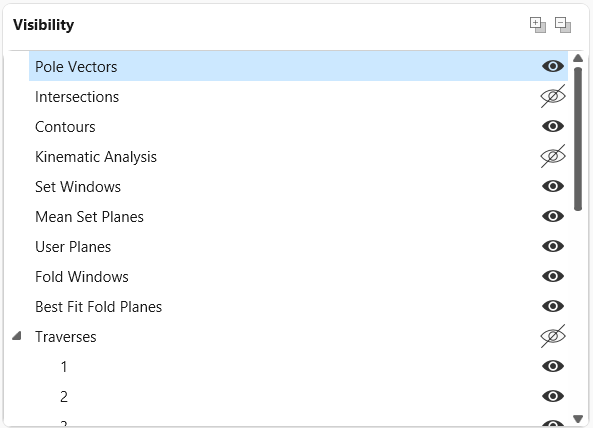
When an entity is selected from the Visibility pane (or graphically, by left-clicking in the view), the associated options (e.g., Color) and entity-specific shortcut options are displayed in the Properties pane.
See the Visibility Pane and Properties Pane topics for more information.
4.2 Projection Pane
The Projection pane allows users to set the Hemisphere (Lower or Upper) and Projection (Equal Angle or Equal Area) type.

See the Projection topic for more information.
4.3 Ribbons
The Stereonet 2D ribbon appears at the top of the application when Stereonet 2D is the active view and provides Stereonet 2D-specific options such as:
- Presets
- User-defined Preset Templates
- Select Poles
- Apply Weighting (Terzaghi Weighting)
- Vector Mode
- User Planes
- Sets
- Slope Kinematics
- Fold Analysis
- Stereonet Overlay
See the Stereonet 2D topic for more information.
The Tools ribbon appears at the top of the application when Stereonet 2D or Rosette is the active view and provides 2D stereonet options for annotations.
See the Tools topic for more information.
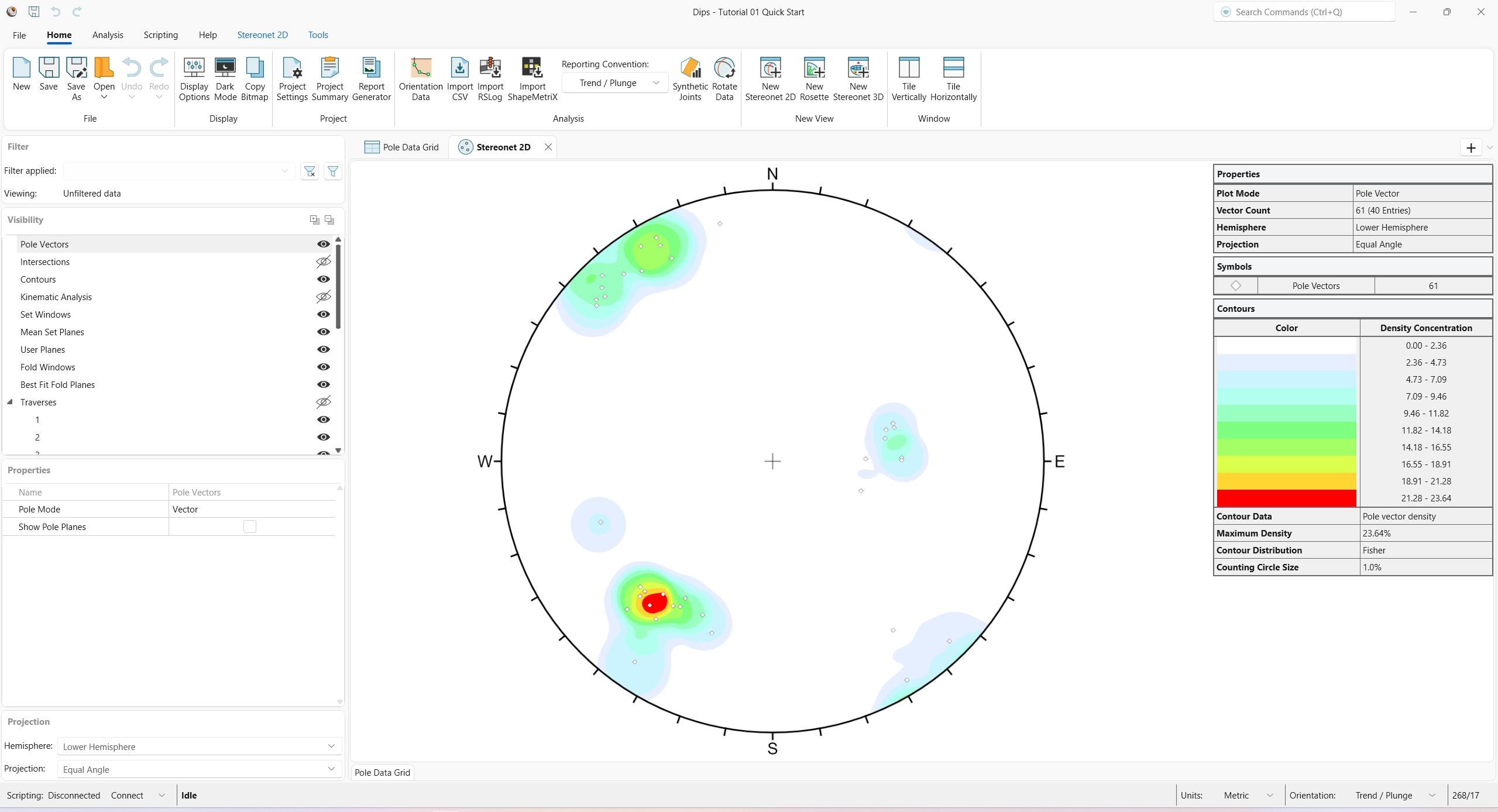
4.4 Vector Plot
The most basic representation of orientation data on a stereonet is the Pole Vector Plot.
- Select Stereonet 2D > Presets > Vector from the ribbon.
- Ensure that Stereonet 2D > Vector Mode > Pole Vector
 is selected from the ribbon.
You should see the following plot.
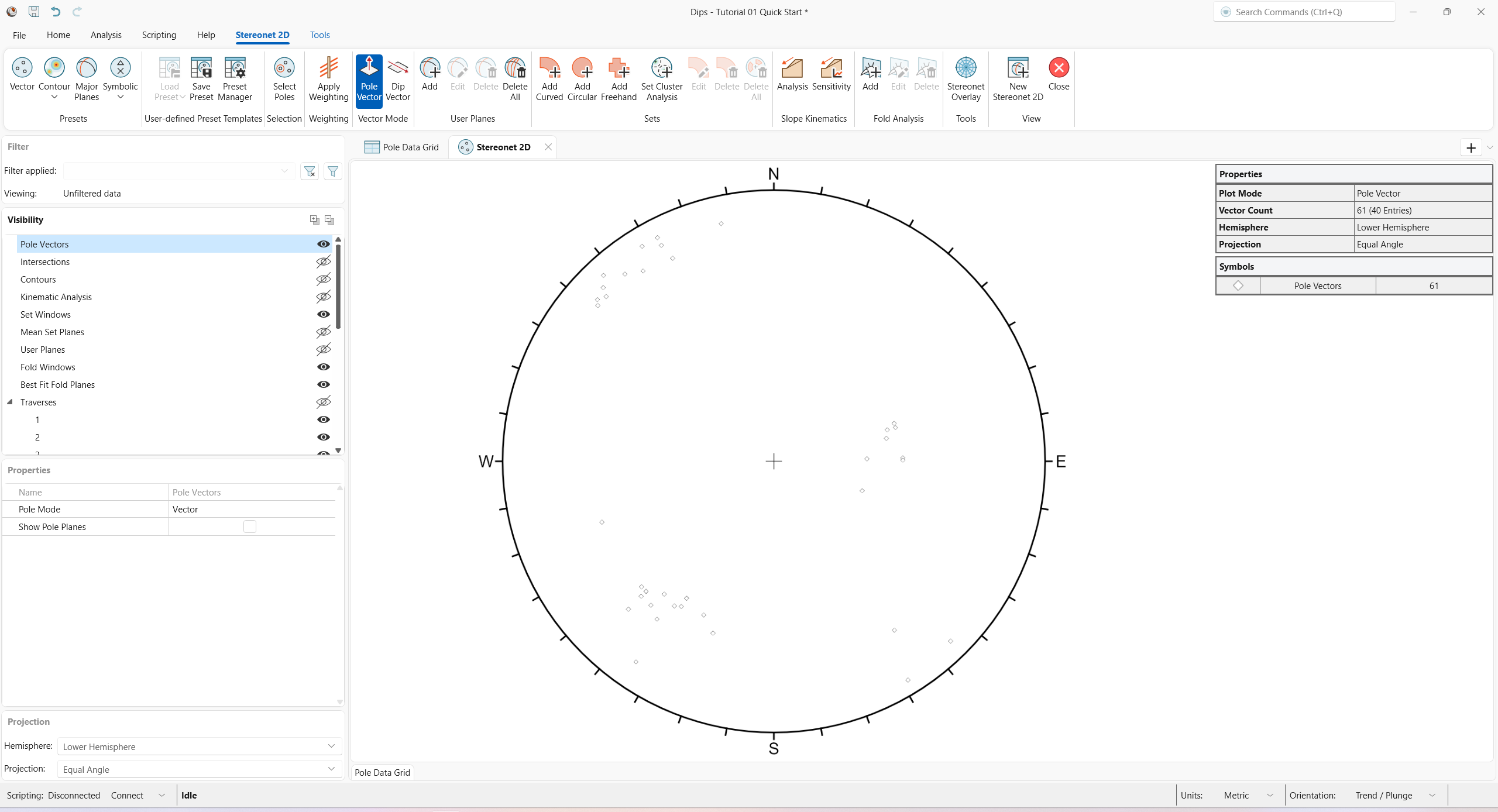
Each pole on a Pole Vector Plot represents an orientation data pair in the first two columns of the Pole Data Grid.
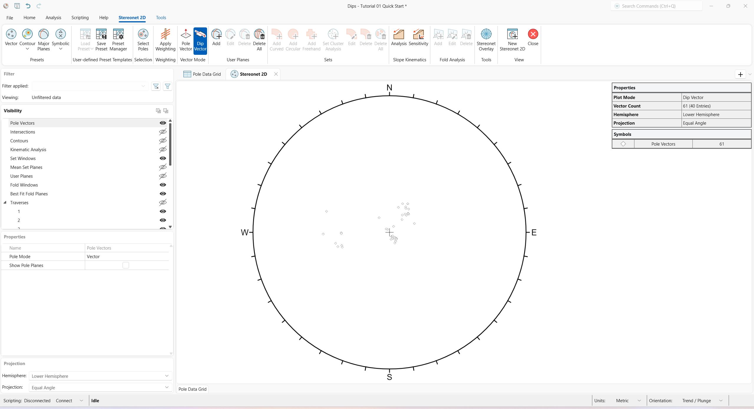
Planes can be represented as either Pole Vectors or Dip Vectors on the stereonet. A Dip Vector Plot represents the maximum Dip orientation of a plane and is orthogonal to the Pole Vector of a plane.
To view Dip Vector Mode:
- Select Stereonet 2D > Vector Mode > Dip Vector
 from the ribbon.
The Stereonet Plot should look as follows.
To return to Pole Vector Mode:
- Select Stereonet 2D > Vector Mode > Pole Vector from the ribbon.
4.5 Show Pole Planes
To display the planes (great circles) for all of the planar data in the Pole Data Grid:
- Select Pole Vectors from the Visibility pane.
- In the Properties pane, select the Show Pole Planes checkbox.
You will see all great circles displayed for all planar entries from the Pole Data Grid, as shown below. Each great circle corresponds to a pole (or dip vector) on the vector plot.
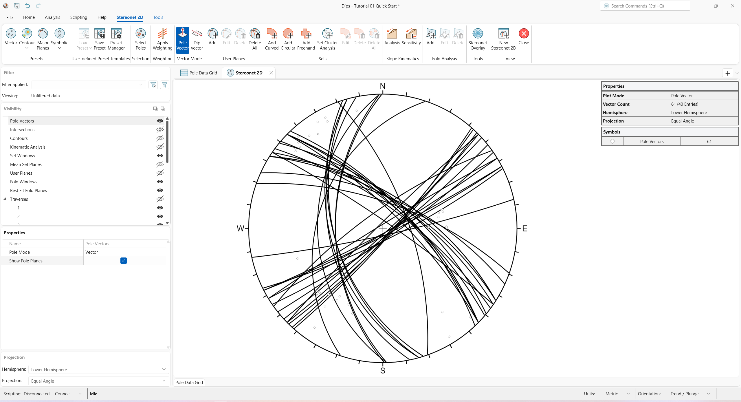
- Deselect the Show Pole Planes checkbox in the Properties pane to turn off the display of Pole Data Grid planes.
4.6 Legend
The Legend pane appears on the right side of the application. Note that the Legend for the Pole Plot (and all Stereonet 2D views) indicates the:
- Properties:
- Plot Mode = Pole Vector
- Vector Count = 61 (40 Entries)
- Hemisphere = Lower Hemisphere
- Projection = Equal Angle
- Symbols:
- Pole Vectors
The Legend pane visibility can be toggled on or off.
- To hide the Legend, hover over the Legend and click on the Legend tab.
- To show the Legend, click on the Legend tab.
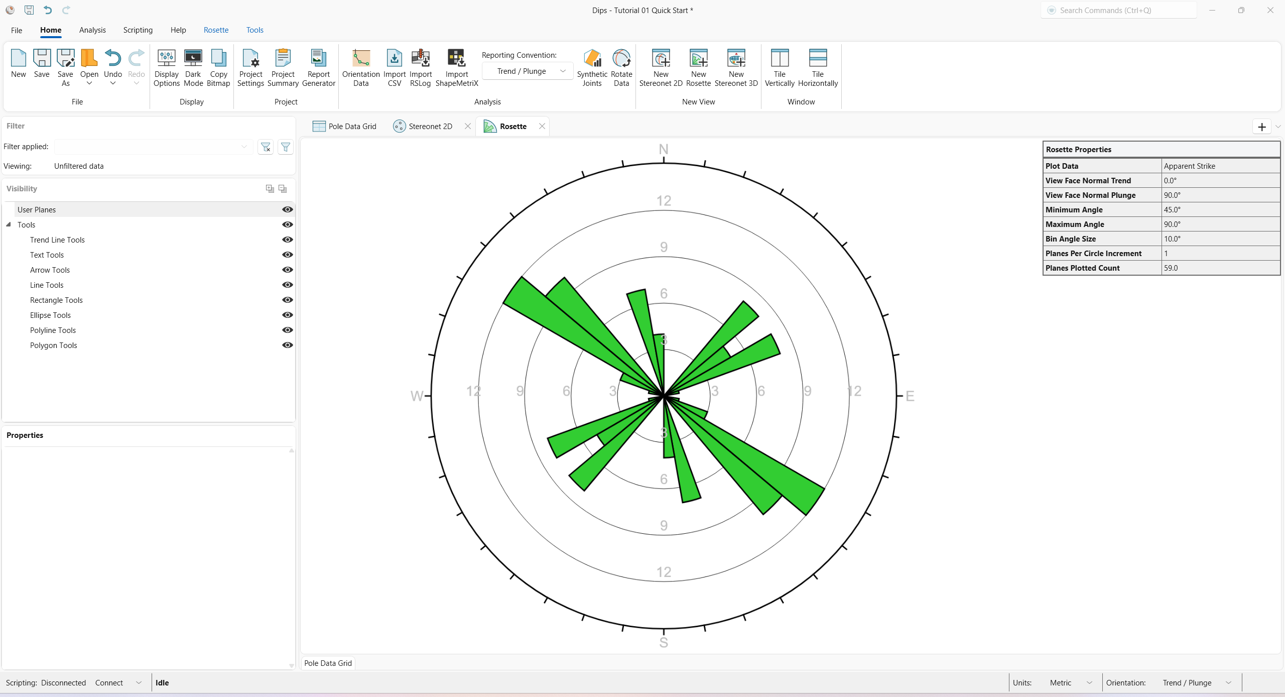
5.0 Rosette
Another widely used technique for representing orientations is the Rosette Plot.
The conventional Rosette Plot begins with a horizontal plane (represented by the equatorial (outer) circle of the plot). A radial histogram (with arc segments instead of bars) is overlain on this circle, indicating the density of planes intersecting this horizontal surface. The radial orientation limits (azimuth) of the arc segments correspond to the range of Strike of the plane or group of planes being represented by the segment. In other words, the rosette diagram is a radial histogram of strike density or frequency.
To open a Rosette view:
- Select Home > New View > New Rosette
 from the ribbon (or New Rosette View from the +
button drop down in the top-right corner of the view tabs)
from the ribbon (or New Rosette View from the +
button drop down in the top-right corner of the view tabs)
A new Rosette view opens.
- Select Rosette > Plot > Plot Options
 from the ribbon.
 - The Rosette Options
dialog appears.
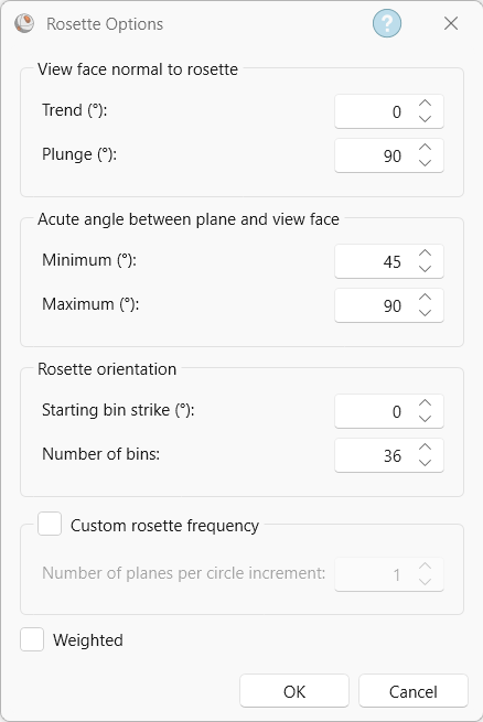
Rosette Options dialog Although the default Rosette Plot uses a horizontal base plane, an arbitrary base plane at any orientation can be specified in the Rosette Options dialog. For a non-horizontal base plane, the Rosette Plot represents the APPARENT STRIKE of the lines of intersection between the base plane and the planes in the Pole Data Grid. - Select Cancel to close the dialog.
See the Rosette Plot and Rosette Options topics for information
5.1 Rosette Applications
The Rosette Plot conveys less information than a full Stereonet 2D view since one dimension is removed from the diagram. In cases where the planes being considered form essentially 2D geometry (prismatic wedges, for example), the third dimension may often overcomplicate the problem. A horizontal rosette diagram may, for example, assist in blast hole design for a vertical bench where vertical joint sets impact on fragmentation. A vertical rosette oriented perpendicular to the axis of a long topsill or tunnel may simplify wedge support design where the structure parallels the excavation. A vertical rosette, which cuts a section through a slope under investigation, can be used to perform quick sliding or toppling analysis where the structure strikes parallel to the slope face.
From a visualization point of view and for conveying structural data to individuals unfamiliar with stereographic projection, rosettes may be more appropriate when the structural nature of the rock is simple enough to warrant 2D treatment.
5.2 Weighted Rosette Plot
The Terzaghi Weighting option can be applied to Rosette Plots to account for sampling bias introduced by data collection along Traverses.
- If the Terzaghi Weighting is NOT applied, the scale of the Rosette Plot corresponds to the actual “number of planes” in each bin.
- If the Terzaghi Weighting IS applied, the scale of the Rosette Plot corresponds to the WEIGHTED number of planes in each bin.
To toggle Terzaghi Weighting:
- Select Rosette > Weighting > Apply Weighting
 from the ribbon to apply Terzaghi Weighting.
 - Deselect Rosette > Weighting > Apply Weighting from the ribbon to remove Terzaghi Weighting.
6.0 Stereonet 3D
A 3D representation of the stereonet is available with the Stereonet 3D view.
To open a Stereonet 3D view:
- Select Home > New View > New Stereonet 3D
 from the ribbon (or New Stereonet 3D from the +
button dropdown in the top-right corner of the view tabs)
from the ribbon (or New Stereonet 3D from the +
button dropdown in the top-right corner of the view tabs)
A new Stereonet 3D view opens.
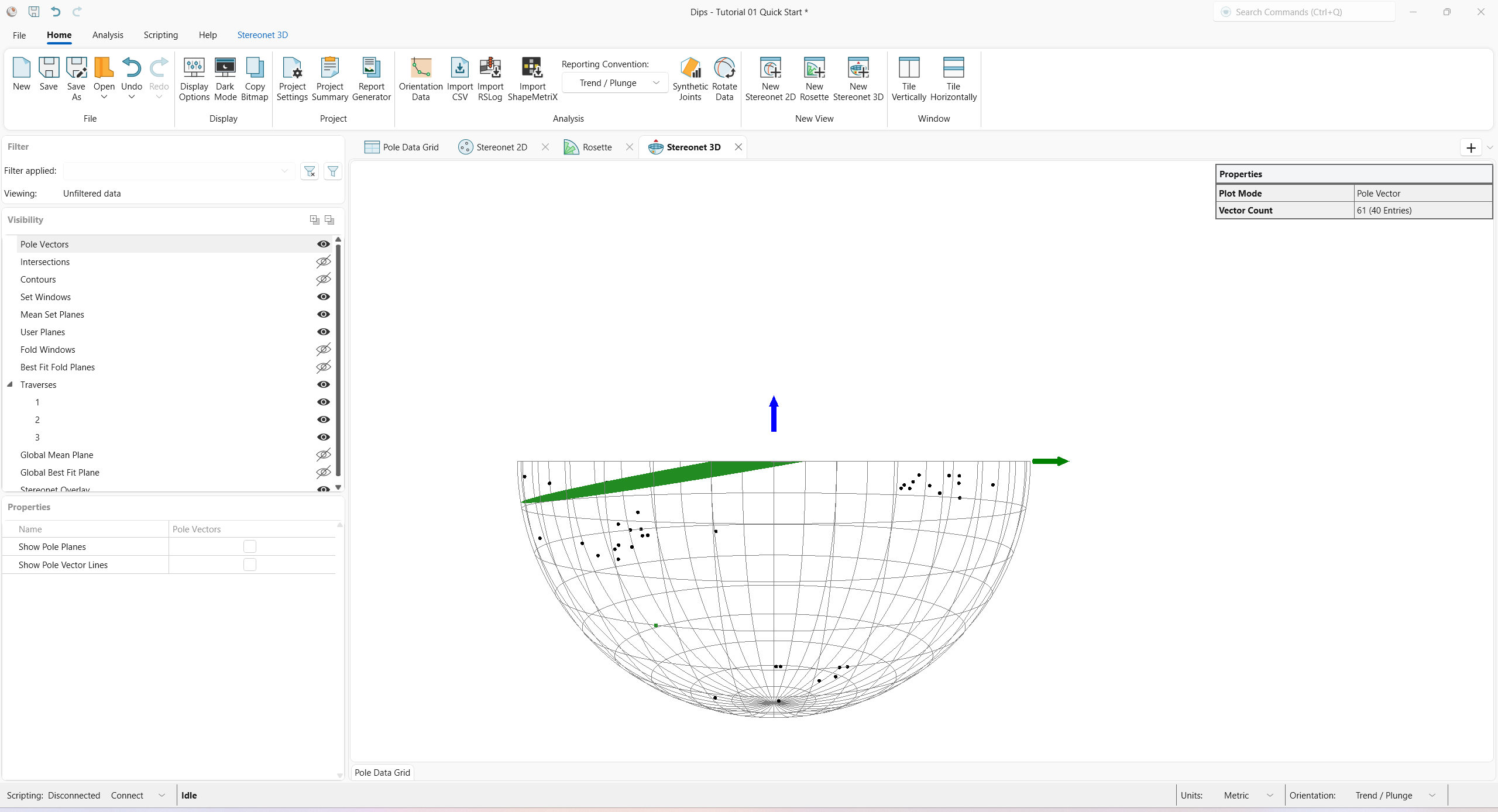
The Stereonet 3D view shows planes as objects in space and plots contours and poles directly on a 3D hemisphere, which helps users to understand how they are related to the 2D projection on the Stereonet 2D.
7.0 Report Generator
The Report Generator is a formatted summary of your DIPS project inputs and analysis results in a ready-to-print report.
- Select Home > Project > Report Generator
 from the ribbon.
 - The Report Generator opens in a separate window.
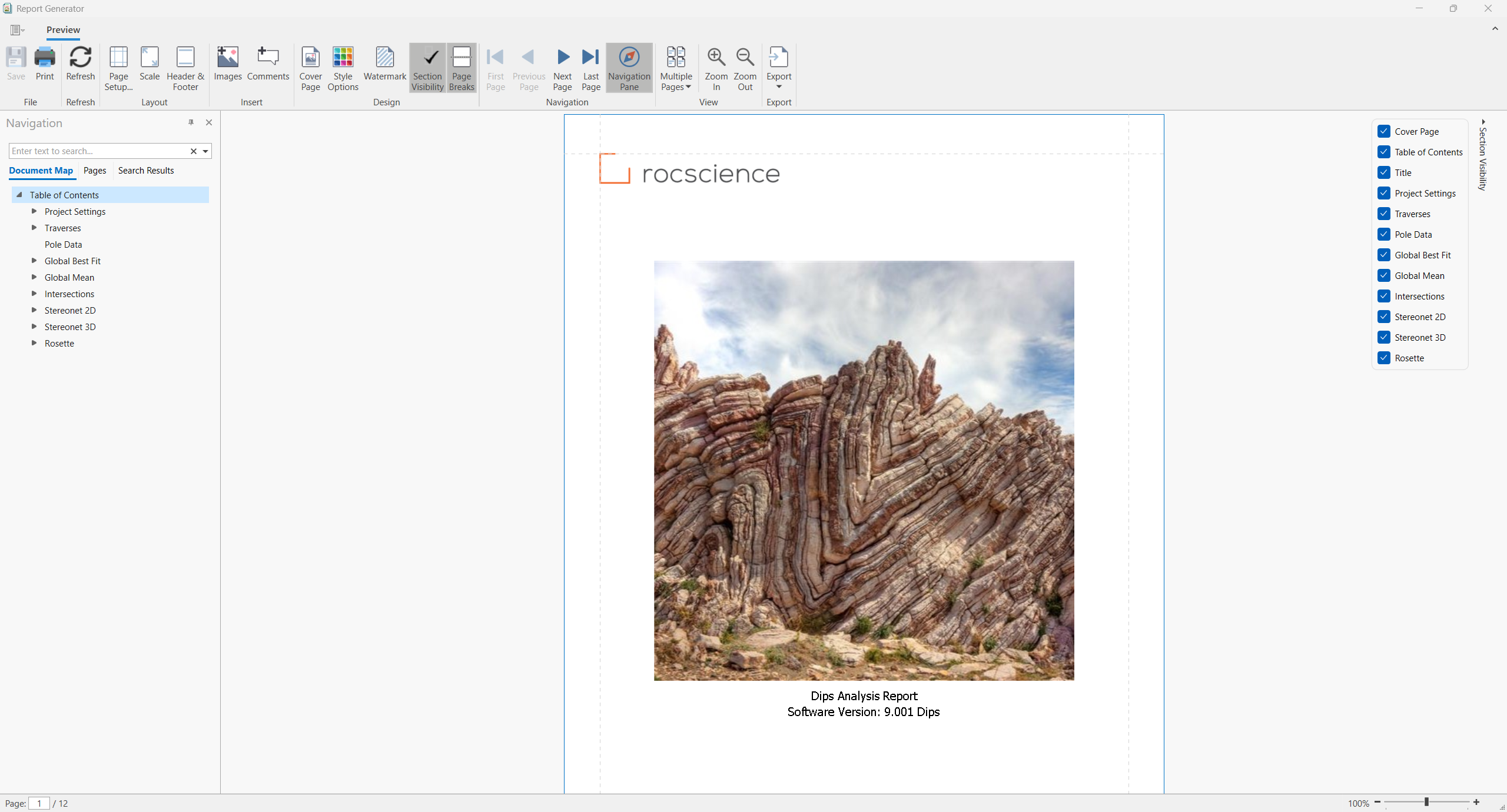
- Various report sections are listed under the Navigation pane to the left of the report window.
- Individual Section Visibility can be toggled on or off.
- The report can be printed with the Print option in the ribbon.
To update the report sections with the latest DIPS changes:
- Select Refresh from the ribbon.
8.0 Working with Multiple Views
Multiple views can be created within a single DIPS project, each with its own view-specific visualization settings.
Views can be:
- Docked or undocked by left-clicking and dragging the view tab (or right-clicking on the view tab and selecting Dock or Float)
- Tiled by selecting Home > Window > Tile Vertically
 or Home Window > Tile Horizontally
  from the ribbon.
This concludes the tutorial. You are now ready for the next tutorial, Tutorial 02 – Curved Set Windows.