12 - Baecher DFN Wizard
1.0 Introduction
This tutorial demonstrates how to generate a Discrete Fracture Network (DFN) from an existing DIPS file using the Baecher DFN Wizard.
Topics Covered in this Tutorial:
- Rock Mass
- DFN Wizard
Finished Product:
The finished products of this tutorial can be found in the Tutorial 12 Baecher DFN Wizard – Finished.dips9 file, located in the Examples > Tutorials folder in your DIPS installation folder.
2.0 Model
If you have not already done so, run DIPS program. To do so:
- Double-click on the DIPS
 icon in your installation folder. Or from the Start menu, select Programs > Rocscience > Dips > Dips.
 - If the DIPS application window is not already maximized, maximize it now, so that the full screen is available for viewing the model.
This tutorial will use the Tutorial 12 Baecher DFN Wizard – Starting File.dips9 file. To open this file:
- Select File > Recent > Tutorials Folder

- Select the Tutorial 12 Baecher DFN Wizard – Starting File.dips9 file and click Open.
3.0 Rock Mass
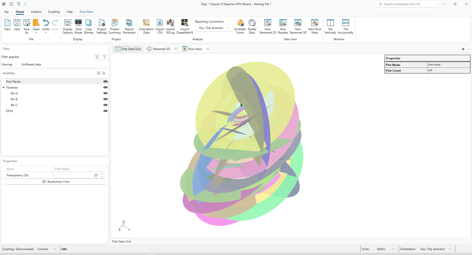
The Rock Mass view displays Linear and Borehole traverses (e.g., Linear Scanline, Linear Borehole Oriented Core, Linear Borehole Televiewer, Curved Borehole Oriented Core, Curved Borehole Televiewer) in 3D space according to their coordinates, as well as the pole planes (i.e., discontinuities) measured along them. The pole planes are plotted as disks with a diameter equal to the value in the Persistence column in the Pole Data Grid. You can also generate and visualize Discrete Fracture Networks (DFNs) in this view.
To open a Rock Mass view:
- Select Home > New View > New Rock Mass
 from the ribbon (or New Rock Mass from the + button drop down in the top-right corner of the screen.)
A new Rock Mass view opens.
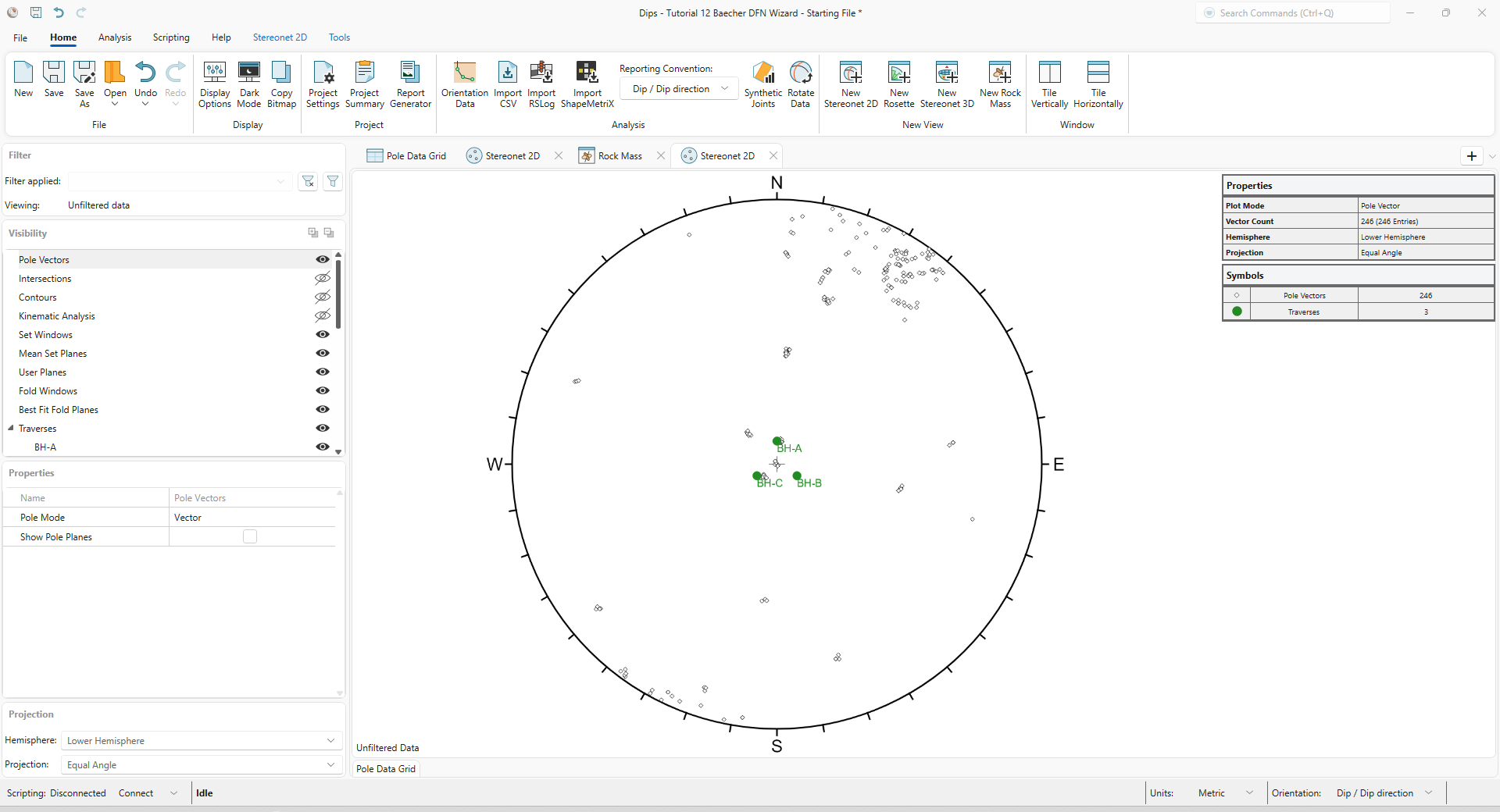
4.0 Stereonet 2D
Open a new Stereonet 2D view:
- Select Home > New View > New Stereonet 2D
 from the ribbon (or New Stereonet 2D from the + button dropdown in the top-right corner of the screen.)
You should see the Steroenet 2D view shown in the following figure.
5.0 DFN Wizard
We will be using the borehole data defined in the Stereonet 2D view to generate a Baecher DFN using the Baecher DFN Wizard.
5.1 Generating a Baecher DFN
To generate a Baecher DFN:
- Select the Rock Mass
 tab to go back to the Rock Mass view.
 - Select Rock Mass > DFNs > Add Baecher DFN
 from the Rock Mass ribbon. This opens the DFN Wizard for generating a Baecher DFN.
 - The Setup section the Baecher DFN Wizard is where you define the bounding region (i.e., box) within which fractures will be generated. The box will be displayed in the Rock Mass viewport. In the Region of Interest section, select Defined By = Dimensions and the dimensions as follows:
- X = 100 m
- Y = 100 m
- Z = 100 m
- Confirm that the Box center is:
- X = 0.09
- Y = 3.51
- Z = 40.25
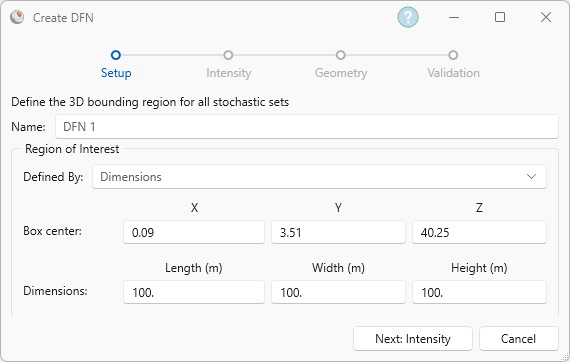
3D bounding region (box) for the DFN If there is data displayed in the viewport, then the bounding region should encompass the data you want to use for DFN generation. Click Next: Intensity to move to the Intensity section.
- We are defining the fracture intensity for DFN Set 1. Under Data source, select Set = None (all data). We will use all the data to define this stochastic set.
- Under Intensity measure, select Method = P10. We will use P10 to define the fracture intensity of this stochastic set.
- P10 zones need to be defined when using P10 as the intensity measure. Click Define P10 zones to open the Define P10 zones dialog.
- In the Define P10 zones dialog, select BH-A
and click Add. This will add a zone to the Cumulative Fracture Intensity (CFI) plot of BH-A that represents the entire borehole. The start depth, end depth, and P10 (i.e., fracture frequency) of that zone are shown in the table underneath the CFI plot.
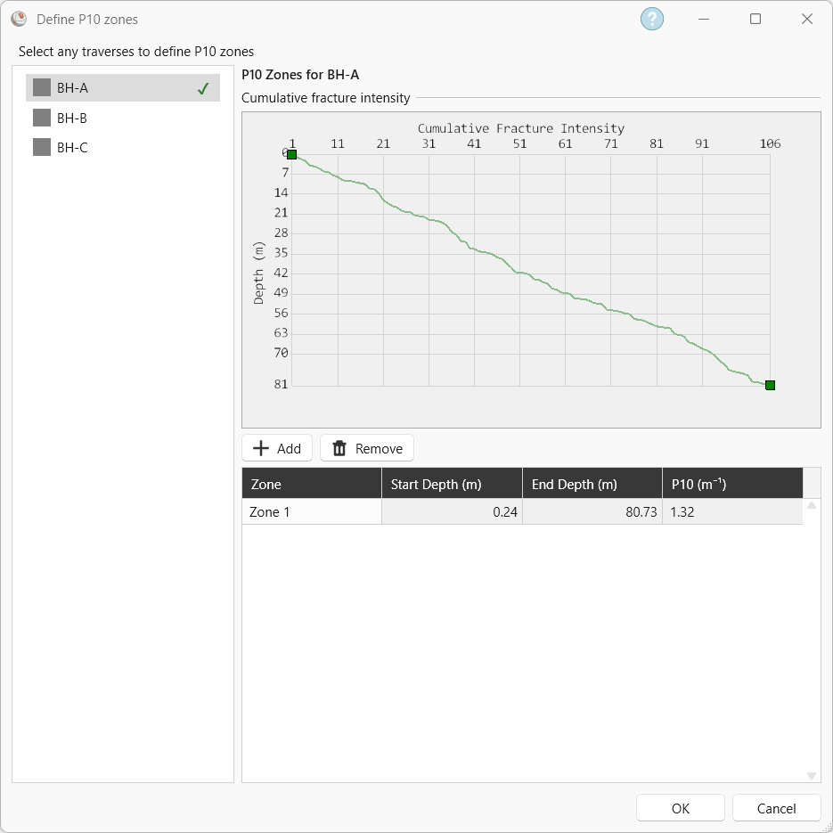 P10 zones are intervals along a borehole’s CFI plot where the slope is constant. Multiple P10 zones can be defined for a borehole if there are variations in the slope; however, it is recommended to use geotechnical domains as the basis for defining P10 zones. P10 zones should not be defined for intervals smaller than a core run length (around 3 m). In this tutorial, the slope of the CFI plot for each borehole is constant, so only one P10 zone needs to be defined for each borehole. Refer to the documentation for more information.
 Repeat the same process for both BH-B and BH-C. The start depth, end depth, and P10 values of their zone are shown in the following table.
Traverse
Zone
Start Depth (m)
End Depth (m)
P10 (m-1)
BH-B
1
0
80.63
0.94
BH-C
1
0.93
79.46
0.81
- Click OK to close the Define P10 zones dialog.
- The table below the Define P10 zones button displays the boreholes with P10 zones and the number of P10 zones.
- When using P10 as the intensity measure, we also need to define the stopping condition. The stopping condition controls when the fracture generation of that set stops. Select First zone from the Stopping condition dropdown.
- The completed Intensity section should look as follows:
Cumulative Fracture Intensity plot with one P10 zone for BH-A 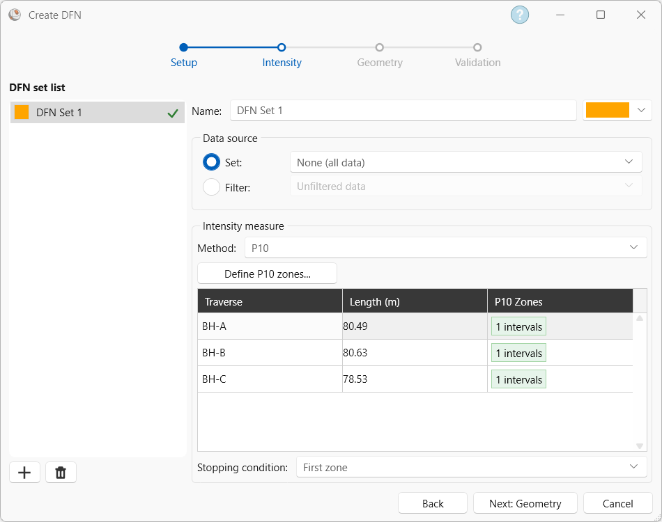 You can define more DFN sets by clicking the + button in the bottom left-hand corner.
- Click Next: Geometry to move to the Geometry section.
- The Geometry section defines the orientation, size, shape, elongation, and rotation of the fractures.
- In the Orientation section, select Distribution = Bootstrap and Noise = 5.Bootstrapping samples directly from the actual orientation data of the selected Set or Filter (including a noise parameter), so that the distribution of the data is preserved in the generated stochastic set.
- In the Shape, set Number of sides = 4. Each generated fracture will have 4 sides.
- The Elongation (ratio) section allows you to specify the aspect ratio of the fracture shape. We will be using the default values in the wizard (the generated fractures will be a square in this DFN):
- Distribution = Constant
- Ratio = 1
- Angle = 0
- In the Size section, select:
- Distribution = Exponential
- Mean = 10 m
- Rel. Minimum = 3 m
- Rel. Maximum = 20 m
- In the context of DFNs, fracture size is not the same as persistence. Fracture size is defined as the radius of a circle with an area equal to the area of the polygon that represents the fracture.
- The Rotation section allows you to specify the rotation of the fracture around its normal. We will be using the default values in the wizard.
- Distribution = Uniform
- Mean = 180°
- Rel. Minimum = 180°
- Rel. Maximum = 180°
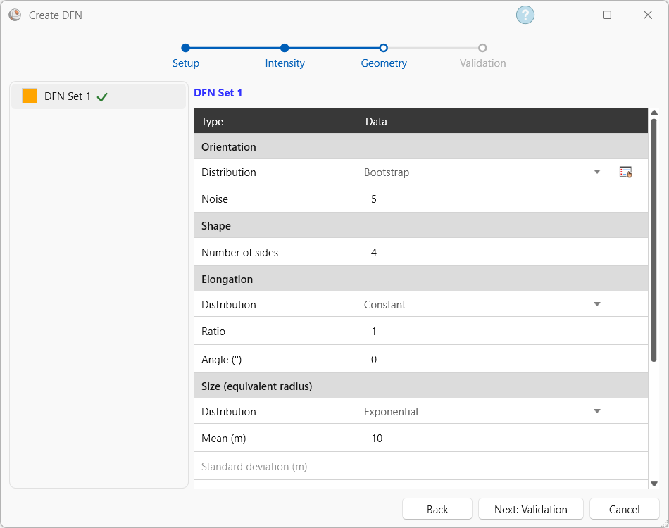
Completed Geometry section of Create DFN dialog. - In the Orientation section, select Distribution = Bootstrap and Noise = 5.
- Click Next: Validation to move to the Validation section.
- In the Validation section, click Preview DFN to preview the DFN in the Rock Mass viewport.The Validation section is meant to preview the DFN and display the Intensity results. It does not imply that the DFN model has been validated against field conditions.
- The Results of the DFN are displayed after Preview DFN is clicked. This shows the actual and simulated P10 or P32 values for each defined zone in a DFN set, as well as total number of fractures. This also shows the total number of fractures and P32 of the whole DFN (all Sets).
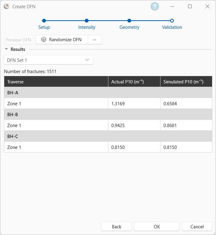
Validation section displaying the results of Set 1 Due to the stochastic nature of the DFN generation process, the results shown above may differ from the results of the model generated by following these steps. - The Validation section also allows you to generate a new realization of the DFN by clicking the Randomize DFN button.
- Click OK to add the DFN to the Visibility Tree and Rock Mass view. The Rock Mass view should look like the following.
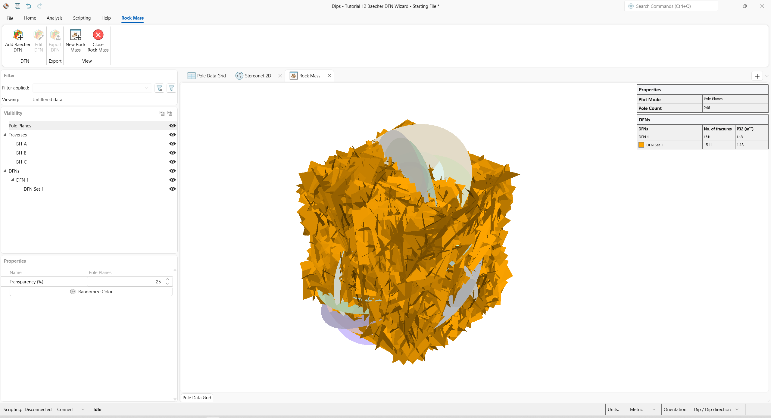
Pole Planes and Generated Baecher DFN Due to the stochastic nature of the DFN generation process, the DFN shown in the figure or in the final model will not exactly match any model generated by following these steps.
- A DFN can be edited by selecting it in the Visibility Tree and clicking Edit DFN
 or exported by selecting it in the Visibility Tree and clicking Export DFN
  in the Rock Mass ribbon.
This concludes the tutorial.