11 - Automatic Cluster Analysis
1.0 Introduction
This tutorial covers the Automatic Cluster Analysis feature in DIPS.
Topics Covered in this Tutorial:
- Automatic Cluster Analysis
Finished Product:
The finished products of this tutorial can be found in the Tutorial 11 Automatic Cluster Analysis (Orientation Data) – Finished.dips9 and Tutorial 11 Automatic Cluster Analysis (Orientation and Quantitative Data) – Finished.dips9 files, located in the Examples > Tutorials folder of your DIPS installation folder.
2.0 Model
If you have not already done so, run the DIPS program. To do so:
- Double-click on the DIPS
 icon in your installation folder. Or from the Start menu, select Programs > Rocscience > Dips > Dips
 - If the DIPS application window is not already maximized, maximize it now, so that the full screen is available for viewing the model.
This tutorial will use the following files:
- Tutorial 11 Automatic Cluster Analysis (Orientation Data).dips9
- Tutorial 11 Automatic Cluster Analysis (Orientation and Quantitative Data).dips9
3.0 Adding Sets (Orientation Data Only)
A Set as defined in DIPS is a grouping of poles created with one of the following options in the Set menu:
- Add Set Window
- Add Set Freehand
- Add Set Circular
- Sets from Cluster Analysis
- Automatic Cluster Analysis
Sets are created for the purpose of obtaining Mean Set Plane orientations and Set Statistics of data clusters.
Sets can be automatically determined with the Automatic Cluster Analysis option. This option uses Fuzzy Cluster Analysis to identify clusters (i.e., sets) from orientation data, as well as quantitative and qualitative rock mass characterization data. The following is just a quick demonstration of identifying sets from orientation data; for further information, see the Automatic Cluster Analysis topic.
- Select Files > Recent Folders > Tutorials Folder
 from the menu.
 - Open the Tutorial 11 Automatic Cluster Analysis (Orientation Data).dips9 file.
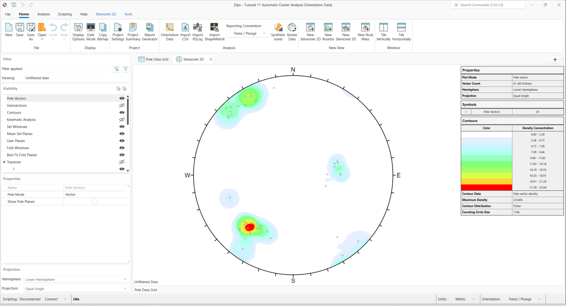
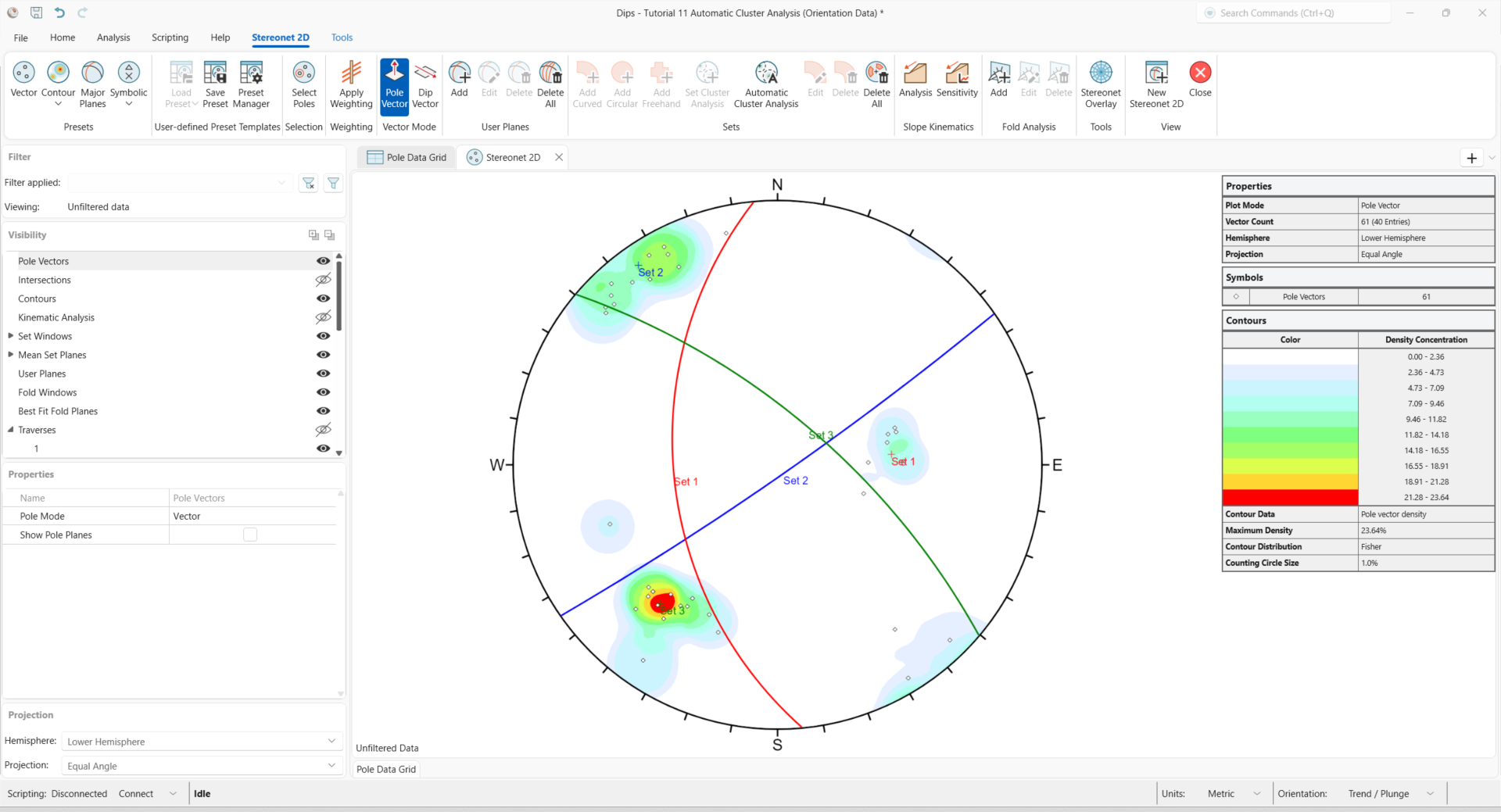
You should see the stereonet plot view shown in the following figure.
If you do not see the plot below, go to the Visibility pane and turn on the visibility for Pole vectors and Contours on the Stereonet 2D View.
- Select Home > Project > Project Settings
 to open the Project Settings dialog.
 - Tick the check box for Use automatic cluster analysis.
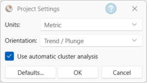
Project Settings dialog with Units set to Metric, Orientation set to Trend / Plunge, and Use automatic cluster analysis is selected - Click OK.
- Select Stereonet 2D > Sets > Automatic Custer Analysis
 . This will open the Automatic Cluster Analysis wizard.
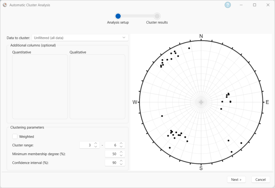
 - For the Analysis setup, enter:
- Data to cluster = Unfiltered (all data)
- We will go over clustering additional data using the Additional columns (optional) option in the next section.
- Weighted = OFF
- Cluster range is between 3 and 6.
- Minimum membership degree (%) = 50
- Confidence interval (%) = 90
The stereonet displays the poles corresponding to the data selected in Data to cluster.
- Click Next. This will perform the cluster analysis.
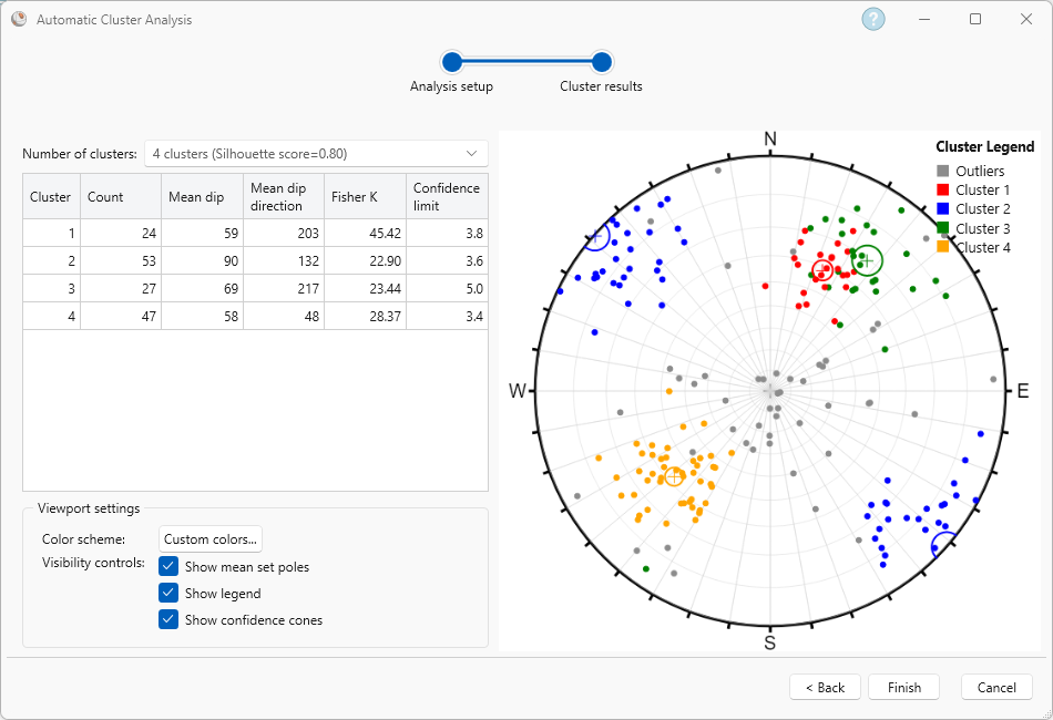
- After clustering is complete, the Cluster results shows:
- The Number of clusters drop down. This drop down shows the number of clusters corresponding to the Cluster range previously set in the Analysis setup. The quality of the cluster results is shown in the Silhouette score for each number of clusters. Toggling through the number of clusters in the drop down will update the set statistics table and the stereonet.
- The set statistics table shows the number of poles, mean set plane dip and dip direction, Fisher K, and confidence limit of each cluster or set.
- The stereonet displays the cluster results. The results are colour coded; the poles, mean set pole, and confidence cone of each cluster are the same colour.
- The colour scheme can be changed by clicking the Custom colors… button or by right-clicking in the stereonet.
- The mean set poles, confidence cones, and legend can be turned ON or OFF with the Visibility controls or by right-clicking in the stereonet.
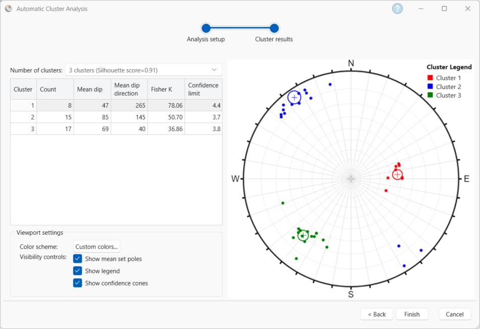
For this data, 3 clusters provides the best results (highest Silhouette score).
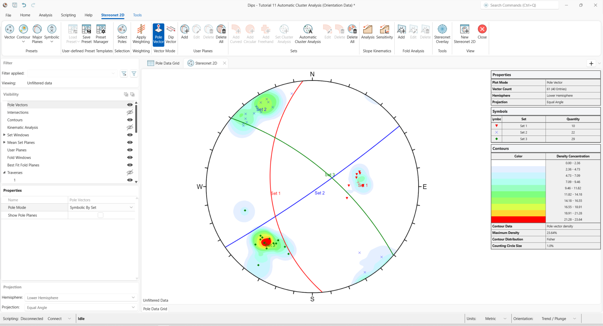
- To apply these cluster results, click Finish. Your screen should look as follows:
The colours of the mean set planes match the colours selected in the wizard.
To plot the poles by their set association:
- In the Visibility pane select Pole Vectors.
- In the Properties pane change Pole Mode to Symbolic By Set. The poles in each set will be displayed in the same colour as their mean set plane.
Notice that Set Windows are not displayed when using the results from Automatic Cluster Analysis. Additionally, mean set planes created from the Automatic Cluster Analysis option CANNOT be edited or individually deleted after they are created. If you need to change the mean set planes, you will have to delete ALL the mean set planes and repeat the clustering process until the results are satisfactory.
4.0 Adding Sets (Orientation and Quantitative Data)
Relying solely on orientation data for discontinuity set identification can result in missing important sets, such as faults and subjoints (where the orientations are similar, but the sets differ by another discontinuity property). The Automatic Cluster Analysis Wizard can use orientation, quantitative, and qualitative rock mass characterization data (such as joint spacing, length, etc) to identify discontinuity sets.
- Select Files > Recent Folders > Tutorials Folder from the menu.
- Open the Tutorial 11 Automatic Cluster Analysis (Orientation and Quantitative Data).dips9 file.
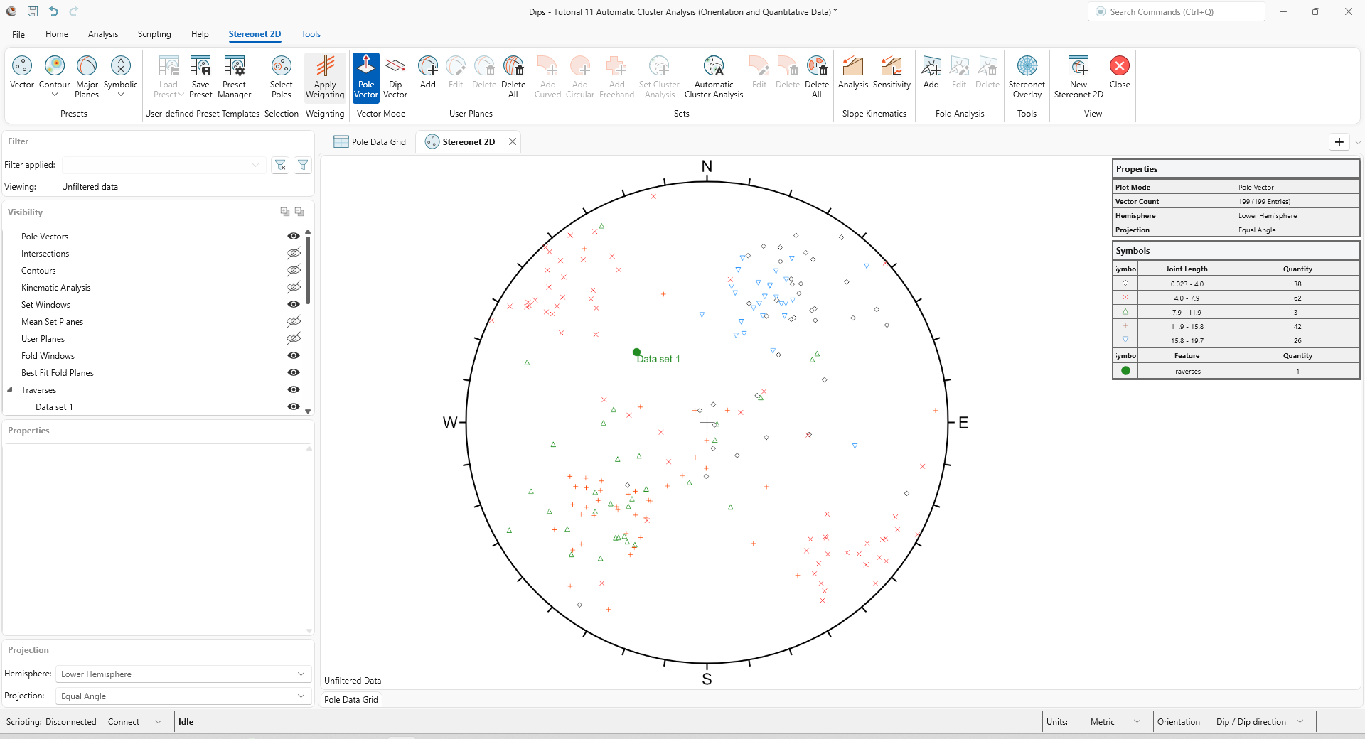
You should see the stereonet plot view shown in the following figure.
If you do not see the plot below, go to the Visibility pane and turn on the visibility for Pole Vectors and Contours in the Stereonet 2D View.
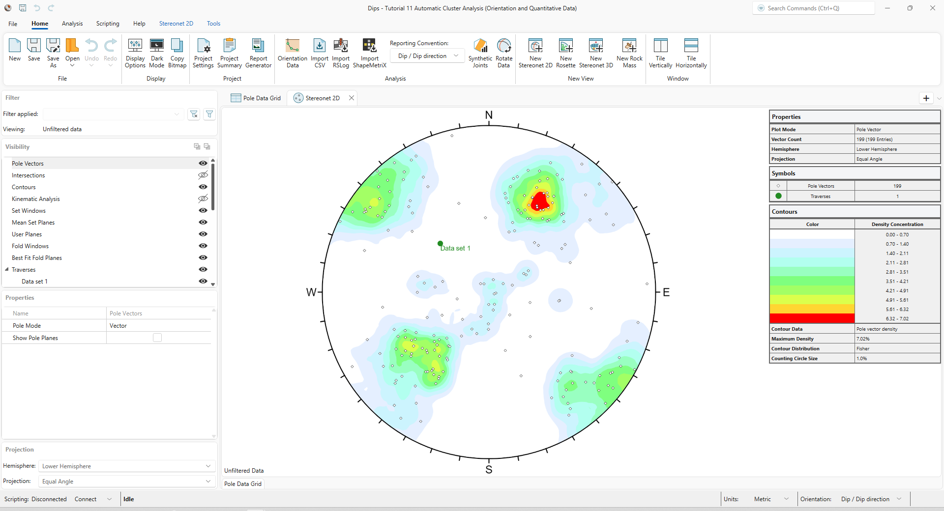
In the Pole Data Grid tab, you will see that a quantitative extra column is available (Joint Length (m)). This column will help us distinguish between overlapping sets.
- Select Home > Project > Project Settings to open the Project Settings dialog.
- Tick the checkbox for Use automatic cluster analysis.
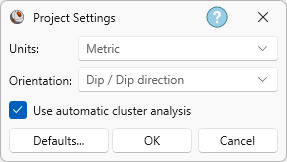
Project Settings dialog with Units set to Metric, Orientation set to Dip / Dip direction, and Use automatic cluster analysis is selected. - Click OK.
We are first going to examine the stereonet. When looking at the contoured stereonet (with or without Terzaghi weighting applied), we can see that there are 3 areas of high-density concentration. However, when we plot a Symbolic Plot of Joint Length (m), we can see that the concentration of poles in the NE corner consists of two distinct joint lengths. This suggests that this concentration of poles may consist of two overlapping sets, instead of one set. To make the symbolic plot:
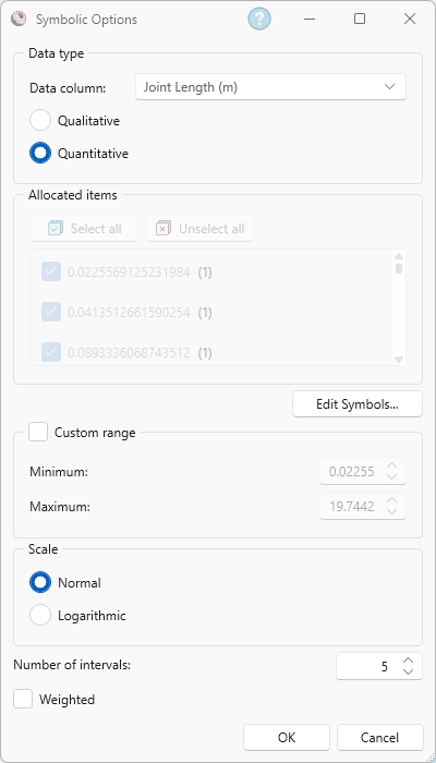
- Select Stereonet 2D > Presets > Symbolic > Symbolic Options

- In the Symbolic Options dialog:
- Set Data column = Joint Length (m)
- Select Quantitative.
- Ensure that Custom range is not selected.
- Ensure Scale = Normal.
- Set Number of intervals = 5
- Weighted is deselected.
The symbolic plot on the stereonet should look as following.
- We are going to first run the analysis using only orientation data. Select Stereonet 2d > Sets > Automatic Cluster Analysis to open the Automatic Cluster Analysis wizard.
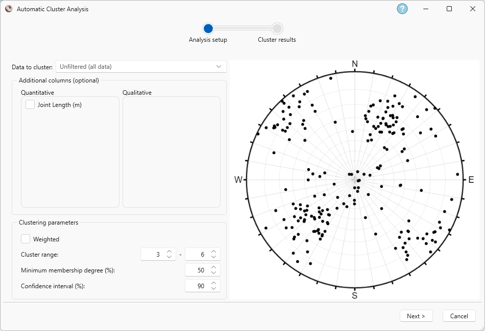
- For the Analysis setup enter the following:
- Data to cluster = Unfiltered (all data)
- Leave Additional columns (optional) deselected.
- Leave Weighted unchecked.
- Cluster range is 3 - 6.
- Minimum membership degree (%) = 50
- Set Confidence interval (%) = 90
The stereonet displays the poles corresponding to the data selected in Data to cluster.
- Click Next. This will perform the cluster analysis.
- After clustering is complete, the Cluster results shows:
- The cluster results with the highest Silhouette score is 4 clusters (0.78). However, these results do not differentiate between poles with similar orientation but different joint lengths (the poles in the NE corner). This is also shown in the other cluster results.
- Click Back to go back to the Analysis setup.
- Under Additional columns (optional) select Joint Length (m). Keep the remaining inputs unchanged.
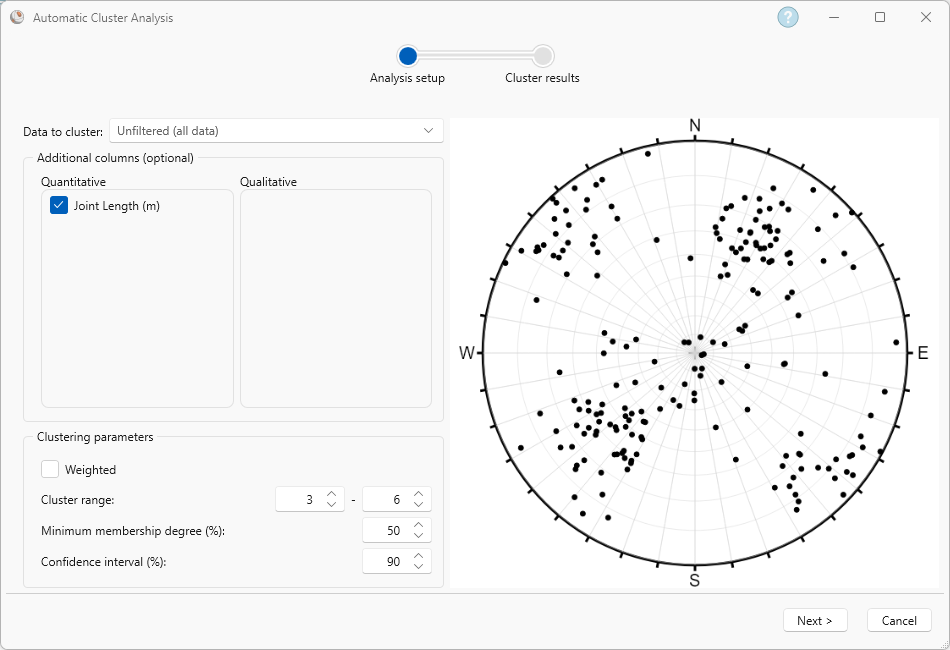
- Click Next. The clustering algorithm will now cluster orientation and joint length data.
- After clustering is complete, the Cluster results shows:
- The cluster results with the highest Silhouette score (0.80) is 4 clusters.
- The results for 4 clusters identified two overlapping sets in the NE corner; these sets have similar orientation but different joint lengths, as seen in the symbolic plot for joint length.
This concludes the tutorial. You are now ready for the next tutorial, Tutorial 12 – Baecher DFN Wizard in DIPS.