14 - Groundwater Flow in Cofferdam

1.0 Introduction

In this tutorial, we will determine the quantity of seepage entering a cofferdam using finite element groundwater seepage analysis in Slide2. This example is based on problem 2.3 from Craig (2012) in which the seepage quantity entering a cofferdam was calculated.

We will construct the problem and solution entirely with Slide2.

Finished Product:

The finished product of this tutorial can be found in File > Recent Folders > Tutorials Folder > Tutorial 14 Groundwater Flow in Cofferdam.slmd.

2.0 Model Geometry

Before we import the geometry, we will set the groundwater analysis option to the finite element analysis method in the Project Settings dialog.

1. Select Analysis > Project settings to open the Project Settings dialog.
2. Under the General tab, make sure the Units of measurements are set to Metric.
3. Set Time Units as Seconds.
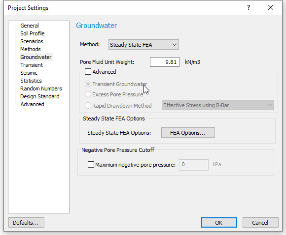
4. Click on the Groundwater tab on the left side of the dialog. Select Steady State FEA as the method. This enables steady-state Finite Element Analysis of groundwater flow. (We will leave the number of iterations and tolerance at their default values specified under the FEA options.)



5. Click OK to save the settings and exit the dialog.

We now have a Slope Stability tab and the Steady State Groundwater tab at the bottom of the viewing window of Slide2.

5. Select File > Import > Import DXF, and open Tutorial 14 Groundwater Flow in Cofferdam.dxf.
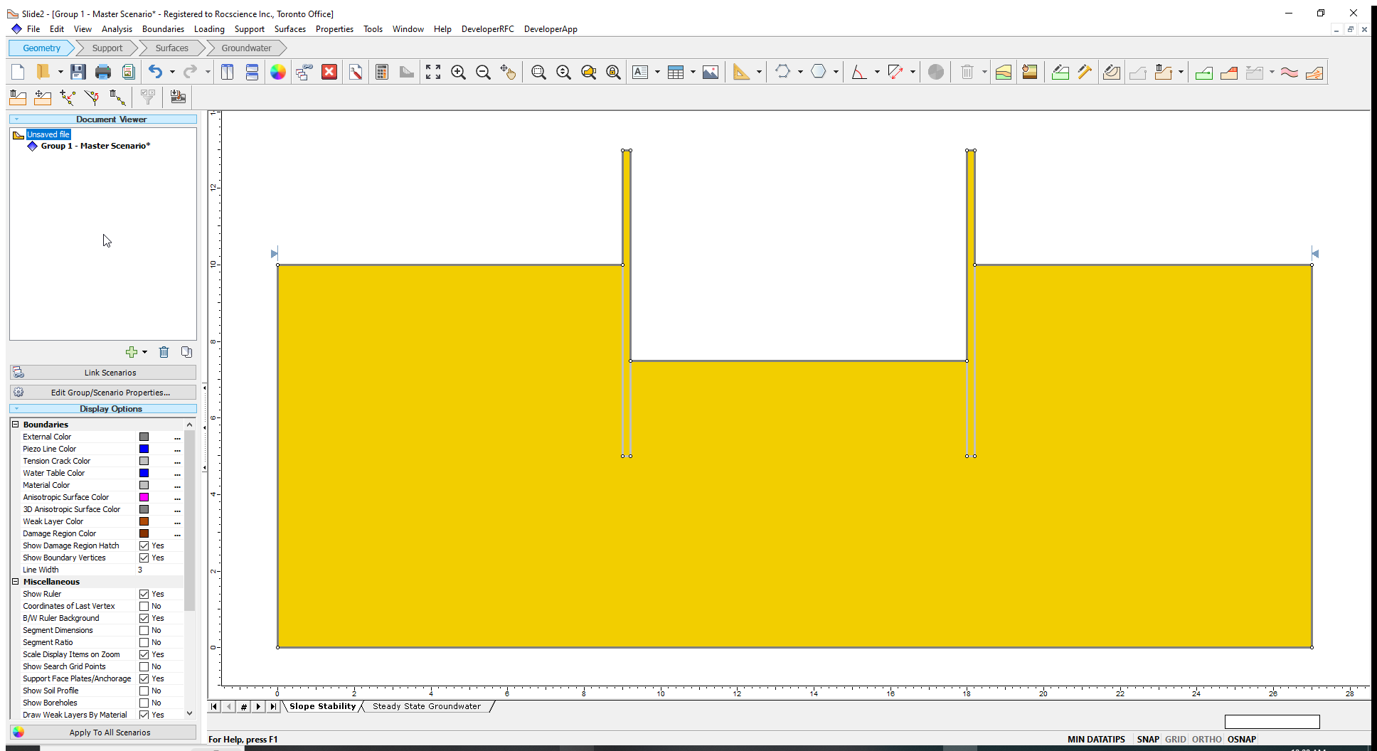
6. The external and material boundaries are correctly assigned. Click OK to import the model as shown below.

Now we will define the material properties.

3.0 Material Properties

1. Go to Properties > Define Materials to open the Define Material Properties dialog.

Since we are only looking at groundwater flow, the material properties don’t matter – we will keep the default properties but change the names of the materials.

2. Select Material 1 and rename it as ‘Soil’. Keep the default material properties.
3. Select Material 2 on the left side of the dialog and rename it to ‘Sheet Pile’.
4. Click OK to close the dialog.

3.1 Assigning Material Properties

By default, the entire model is assigned the properties of Soil (Material 1).

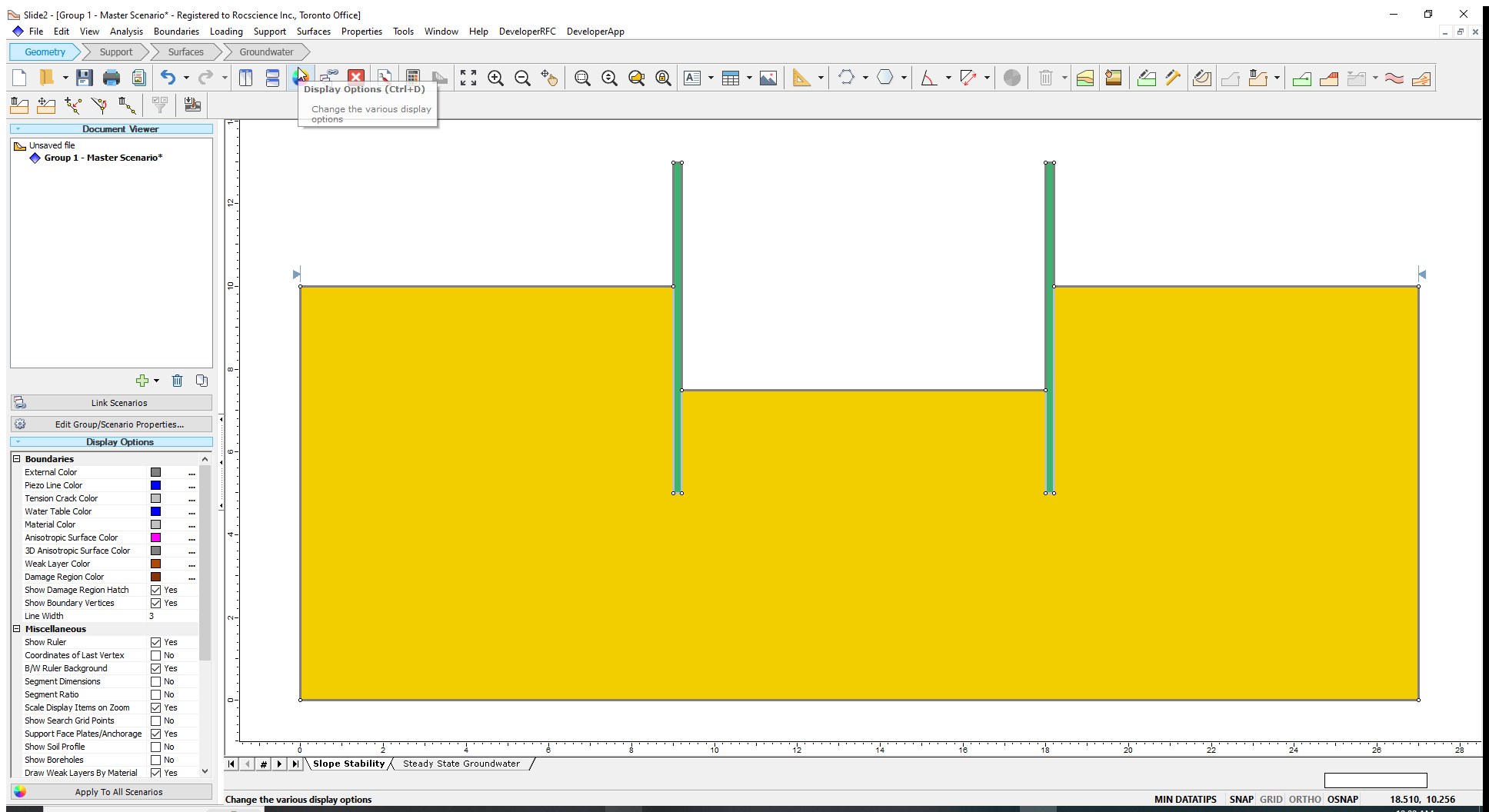
1. Select Properties > Assign Properties to open Assign dialog. Select the Sheet Pile material and then click on each Sheet Pile (the two narrow sections bounding the trench) to assign the material property.
2. Close the Assign dialog. Your model will look as shown:

3.2 Hydraulic properties

Next, we will define the hydraulic flow properties of the soil. To do this, we first need to switch to the groundwater mode. You can do this by selecting Analysis > Steady State Groundwater Mode and using the Groundwater tab at the top, or by clicking on the tab at the bottom of the screen for Steady State Groundwater.

1. Select the Steady State Groundwater tab at the bottom of the screen.
2. Go to Properties > Define Hydraulic Properties
   
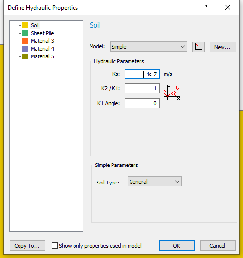
3. For Soil, enter a Ks (Ks is hydraulic conductivity, also known as saturated permeability) value of 4e-7.
4. For the Sheet Pile, enter a Ks value of 1e-20. (The sheet piling is assumed to be essentially impermeable. We cannot choose a permeability of 0 since this will lead to numerical instability, therefore we set the permeability to a very small number.)
5. Do not change any other parameters. (We are assuming that permeabilities are isotropic, i.e., remain the same in all directions.)

The Model option at the top of the Hydraulic Properties dialog refers to the relationship (function of matric suction) used to define permeability in the unsaturated zone. Different models, including user-defined functions, may be specified. However, we will use the default Simple option. See Slide2 Help for more information on permeability models.

6. Click OK to close the dialog.

4.0 Boundary Conditions

Before we can set the boundary conditions, we must generate the finite element mesh. We will use the 6 noded triangles and an approximate number of elements of 1500 to generate the mesh.

1. Select Mesh > Mesh Setup
2. Change the element type to 6 Noded Triangles.
3. Click OK.

To generate the mesh:

4. Go to Mesh > Discretize and Mesh You should see the mesh generated for the model.

Now we can set the boundary conditions.

We will simulate ponded water to the left and right of the sheet piling. We will stipulate a water elevation of 13 m, which equals the elevation of the top of the sheet pile.

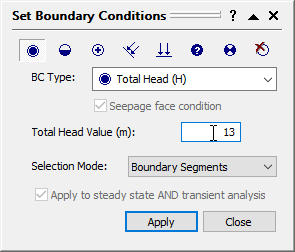
5. Go to Mesh > Set Boundary Conditions to open the ‘Set Boundary Conditions’ dialog.
6. For BC Type choose Total Head.
7. Enter a Total Head Value of 13.
8. Ensure the selection mode is Boundary Segments.
   
   
9. Now select the four boundary segments shown on the image below to define the required ponded water areas of the model. The coordinates of the segments are as follow:
• Line 1: from (0,10) to (9,10)
• Line 2: from (9,10) to (9,13)
• Line 3: from (18.2,10) to (18.2,13)
• Line 4: from (18.2,10) to (27,10)
10. Click Apply to set this boundary condition.

Before we close the Set Boundary Conditions dialog, we will apply zero pore pressure boundary condition to the interior of the coffer dam because it is at atmospheric pressure.

11. Change the BC type to Zero Pressure (P=0) and click on the interior segment: (9.2, 7.5) to (18.0, 7.5).
12. Click on the Apply button to assign the zero-pressure boundary condition and then click Close to exit the dialog.

To calculate the flow quantities in the coffer dam, we will define a discharge section.

4.1 Discharge Sections

In Slide2, a Discharge Section is a user-defined polyline segment, across which steady-state, volumetric flow rates, normal to the segments, will be calculated during groundwater seepage analysis.

We will add a horizontal discharge section at the following locations to calculate inflows into the excavation:

• Below the ponded water at both sections of the dam and
• Below the soil surface between the sheet piles.

To do this, proceed as follows:

1. Go to Discharge > Add Section to activate the Prompt line.
2. Enter the first coordinates in the Prompt line (0, 9.5), press Enter, and then enter the second coordinates (9, 9.5) and press Enter.
3. Press Enter again to finish drawing.
4. Repeat steps (1) and (2) to draw two more discharge sections with the following coordinates:
• (18.2, 9.5) to (27,9.5)
• (9.2, 7) to (18, 7)

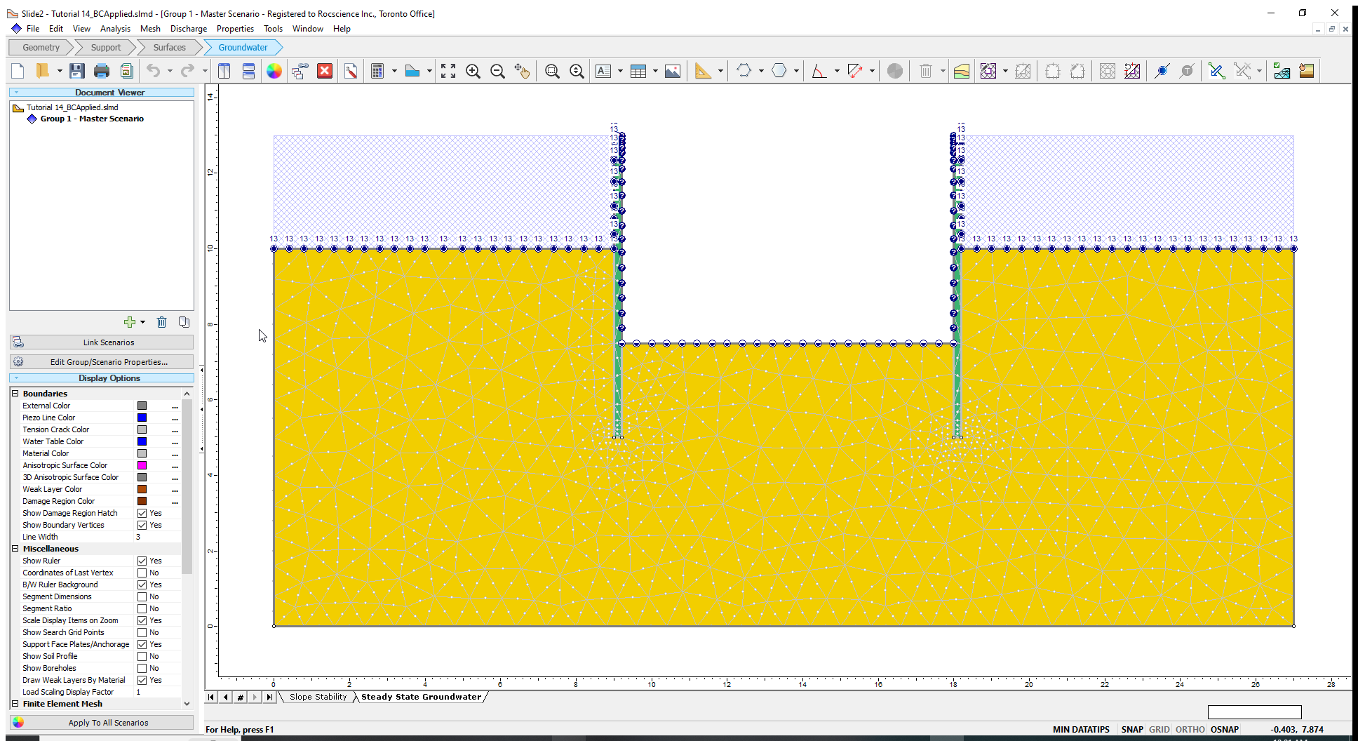
The discharge sections are displayed as green lines, with small circles marking the endpoints. The value of the flow rate across these lines will be displayed in the Slide2 Interpret program.

Your final model should now appear as shown below.

Now we are ready to compute the analysis.

5.0 Computation and Interpretation of Results

Since we are interested in only the groundwater results, we will run the steady state groundwater engine alone.

1. Select Analysis > Compute (groundwater) Click OK in the computation window. The analysis should take a few seconds to run.
2. Go to Analysis > Interpret (groundwater) to view the results when computations are done.

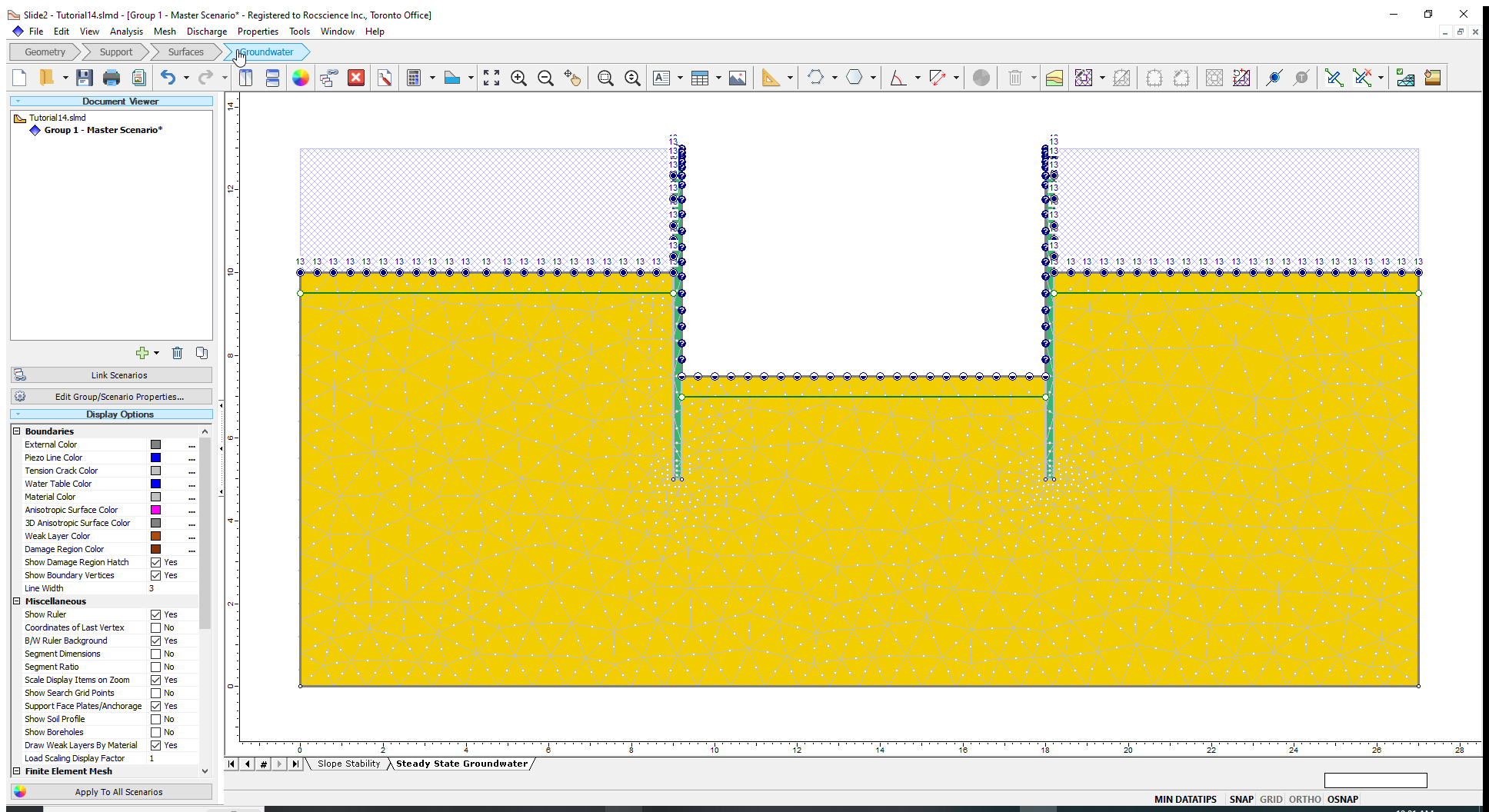
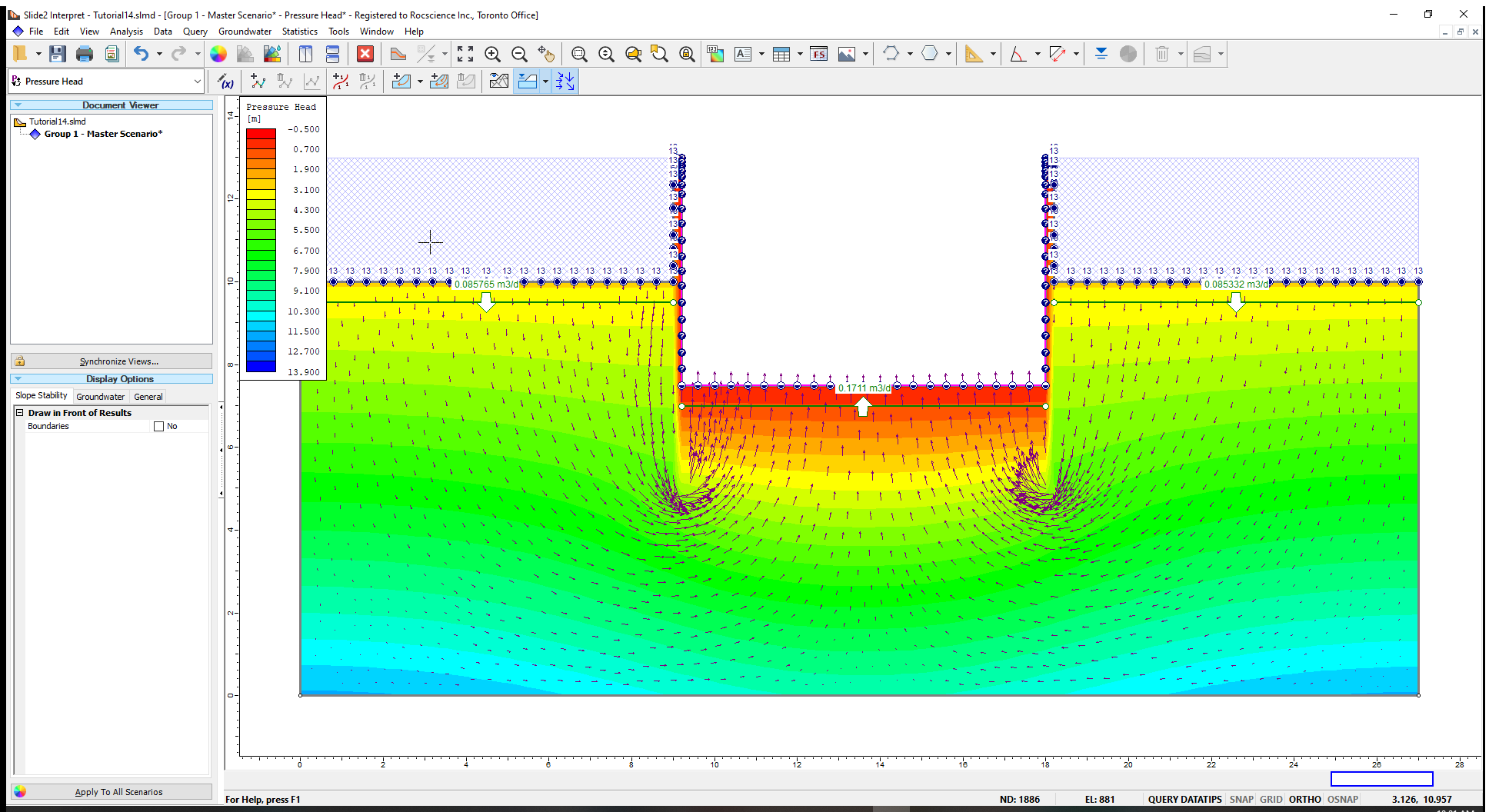
The Pressure Head contours are displayed first in the results shown in the image below.

The volumetric flow rate and direction through each of the discharge sections are also displayed. From the results, we can see that the water is flowing downwards along the sheet pile walls from the ponded water areas and upwards into the excavation.

The volumetric flow into the dam is 1.98e-6 m3/s. The value in Craig’s (2012) is 2.0e-6 m3 /s. The model, therefore, gives the same result within the number of significant digits given. The sum of the volumetric downwards flow is equal to the volumetric upwards flow between the sheet pile walls.

To see the magnitude and direction of flow throughout the model:

3. Click on the Flow Vectors icon in the toolbar.

The flow vectors are displayed on the model as shown in the image below.

The groundwater is flowing around the impermeable sheet pilings with high flow rates directly below the pilings.

We will construct a flow net as was done in the Craig’s solution.

4. Turn off the flow vectors by clicking on the Flow vectors icon again.

First, we will draw the equipotential lines followed by flow lines.

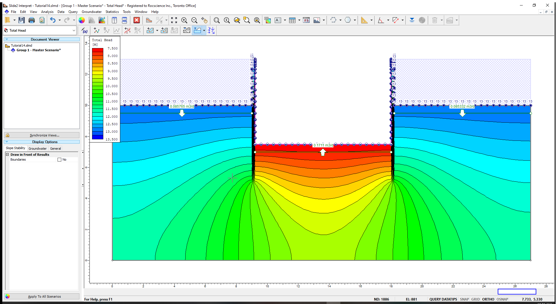
5. In the Data type drop-down, change Pressure Head to Total Head. (Total Head contours represent equipotential lines.)
6. Right-click on the model and select Contour Options to open the dialog.
7. In the Contour Options dialog, change Mode to Filled (with lines).
8. Click Done to close the dialog. The equipotential lines of the flownet are drawn.

We will construct flow lines using the multiple flow lines feature in Slide2.

1. Go to Groundwater > Lines > Add Multiple Flow-Lines
2. Select the top left corner of the coffer dam (0, 10) and move the cursor horizontally until you intersect the sheet pile (9.2, 10) and hit the enter key to open the ‘Flow-Line Start Location’ dialog.
   
3. Under Start Flow-Lines select the first option of locations evenly spaced along the polyline using the default value of 10 locations.
   
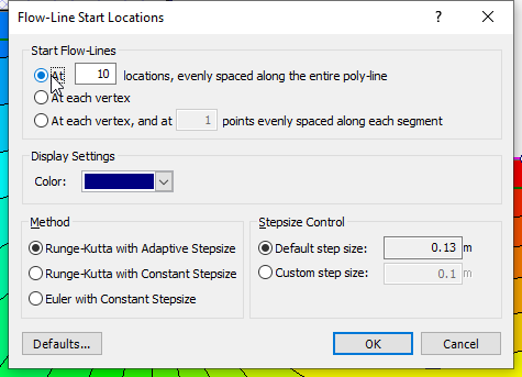
4. Click OK to close the dialog.
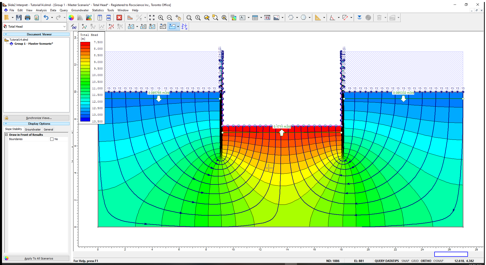
5. Repeat steps (1) and (2) for the right side of the model.
6. The coordinates for the right side are (27,10) and (18,10).

The flow net is drawn as shown below.

6.0 Additional Exercises

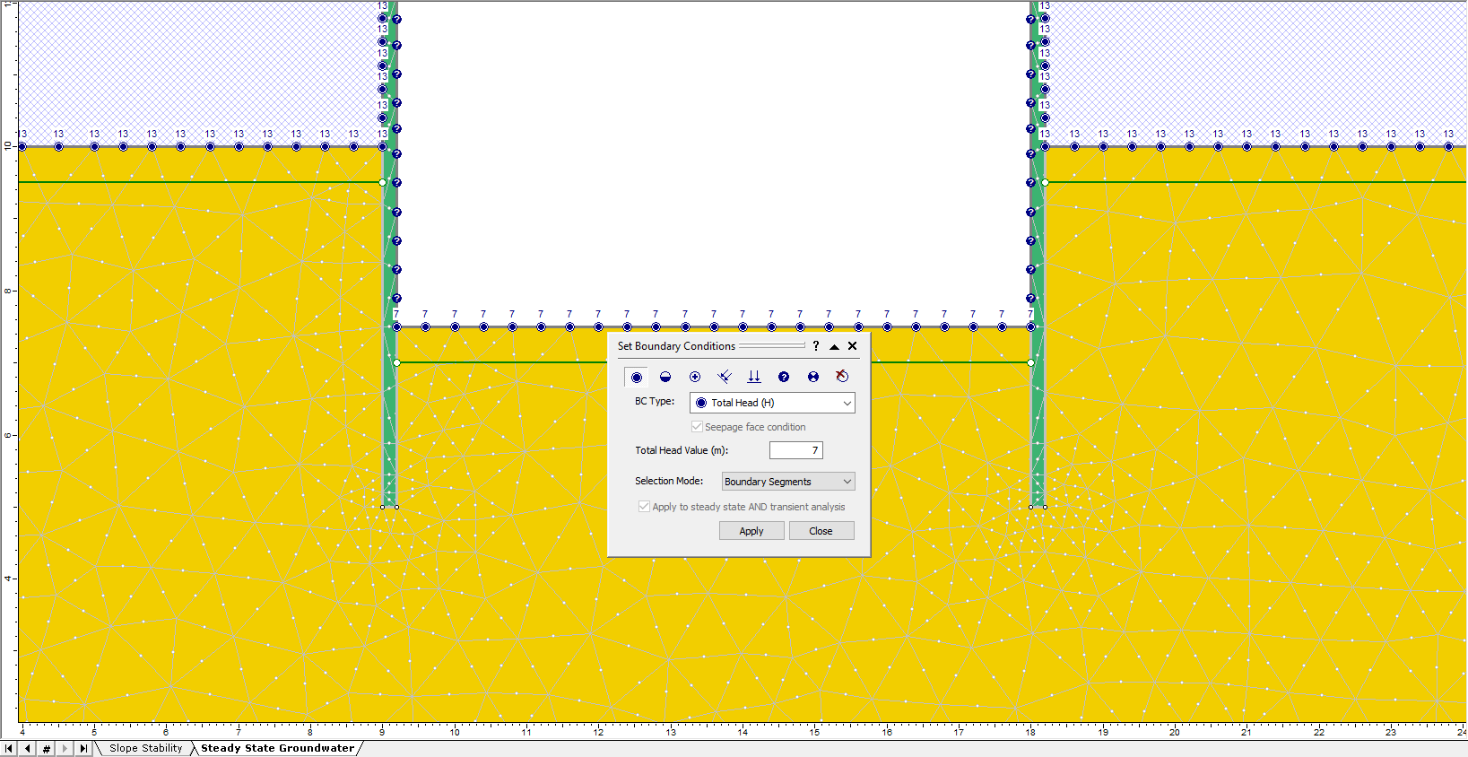
We can simulate pumping at the bottom of the dam by setting a value for total head less than the elevation of the surface.

1. Change the boundary conditions for the bottom of the dam from zero pressure to Total Head = 7 m.
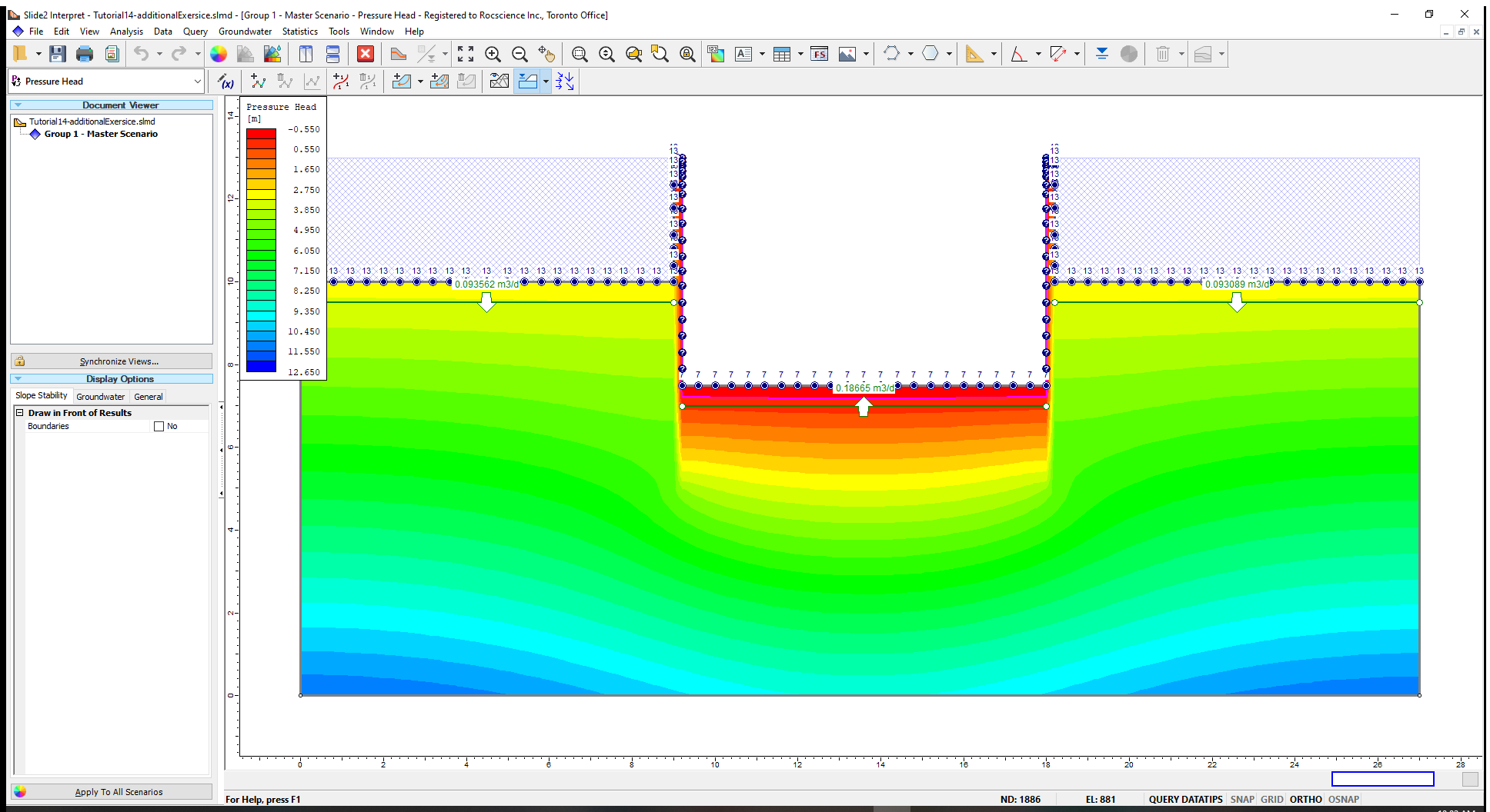
2. Recalculate and plot the results with the Interpret program.

You can see that the volumetric discharge at the bottom of the dam is higher than before. You can also see that the water table has been lowered. The water table is shown as a pink line (your water table line may be obscured by the green discharge line. To hide the discharge line, right-click on it and choose Hide Discharge Sections).

7.0 References

Craig, R.F., 2012. Craig’s Soil Mechanics, 8^th edition, Spon Press, London and New York.