7 - Probabilistic Analysis
1.0 Introduction
This tutorial will familiarize the user with the Probabilistic Analysis features of UnWedge. In a Probabilistic Analysis, you can define statistical distributions for input parameters (e.g., Joint Properties, Field Stress, Water Pressure, Bolt Properties) to account for uncertainty in their values. The computed analysis results in a distribution of factors of safety for each wedge, from which Probabilities of Failure (PF) are calculated.
Topics Covered in this Tutorial:
- Project Settings
- Random Variables
- Fisher Distribution
- Mean Wedges
- Picked Wedges
- Histograms
- Scatter Plots
- Design Factor of Safety
Finished Product:
The finished tutorial can be found in the Tutorial 07 Probabilistic Analysis.weg5 file located in the Examples > Tutorials folder in your UnWedge installation folder.
2.0 Model
- If you have not already done so, run the UnWedge program by double-clicking the UnWedge icon in your installation folder or by selecting Programs > Rocscience > UnWedge > UnWedge in the Windows Start menu. When the program starts, a default model is automatically created.
If the UnWedge application window is not already maximized, maximize it now so that the full screen is available for viewing the model.
2.1 PROJECT SETTINGS
Let's start by configuring basic parameters in the Project Settings dialog.
- Select Projects Settings
 on the toolbar or the Analysis menu.
 - In the General tab, set Analysis Type = Deterministic.
- Make sure Units is set to Metric, stress as MPa.
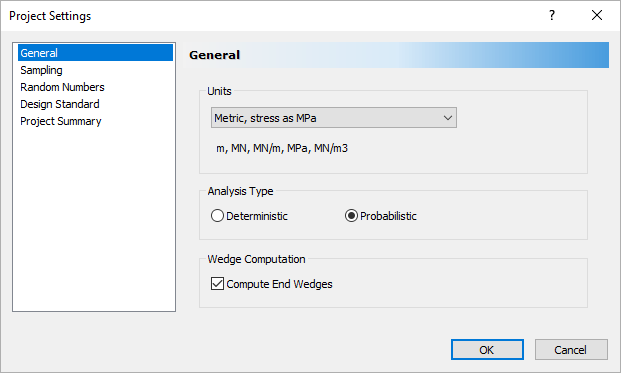
Project Settings General Tab Dialog
2.1.1 Sampling and Random Numbers
- Select the Sampling tab.
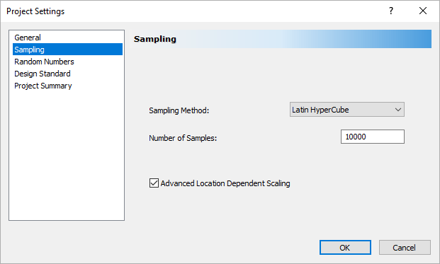
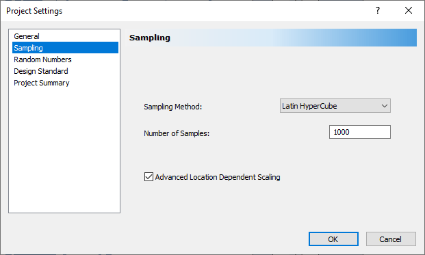
Project Settings Sampling Tab Dialog
The Sampling Method determines how the statistical distributions for the random input variables will be sampled. - Leave the default Sampling Method = Latin Hypercube and Number of Samples = 10,000 as is.
- Select the Random Numbers tab.
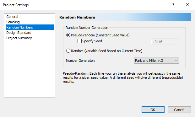
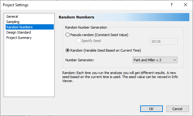
Project Settings Random Numbers Tab Dialog - Do not make any changes in this tab but note that the default for Random Number Generation is Pseudo-Random by default.
This allows you to obtain reproducible results for a Probabilistic Analysis, by using the same “seed” value to generate random numbers. We will discuss Pseudo-random versus Random sampling later in this tutorial.
2.1.2 Design Standards
- Select the Design Standard tab.
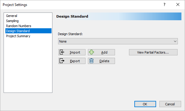
Project Settings Design Standards Tab Dialog - Leave all the settings as is.
Eurocode 7 is a design document that establishes rules and standards for geotechnical engineering design across Europe (BSI, 2004). Eurocode 7 represents a major change in design philosophy. Traditionally a single, lumped Factor of Safety accounts for all of the uncertainties in the problem. With Eurocode 7, partial factors of safety are applied to different components of the analysis. The partial factors are applied prior to the analysis to give design values that are used in the calculation. The final result is an over-design factor, which must be greater than 1 to ensure the serviceability limit state requirement is satisfied. For more information on using Eurocode 7 in geotechnical design, see Smith (2006) and Bond and Harris (2008). This tab allows the user to design using Eurocode 7 specifications.
2.1.3 Project Summary
- Select the Project Summary tab.
- Enter UnWedge Probabilistic Analysis Tutorial as the Project Title.
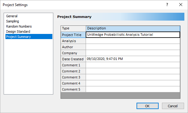
Project Settings Summary Tab Dialog - Select OK to save your settings and close the Project Settings dialog.
2.2 MODEL GEOMETRY
We will start by creating the two-dimensional cross-section of the excavation we want to analyze. The cross-section can either be imported as a DXF file or defined within the program using the Add Opening Section option. For this tutorial, we will use the Add Opening Section option.
2.2.1 Set View Limits
First, we'll set View Limits.
- Make sure Opening Section is selected in the View dropdown on the toolbar.
- Select View > View Limits

The View Limits dialog appears. - Enter 250, 300 for the Minimum X, Y Coordinates and 280, 300 for the Maximum X, Y Coordinates.
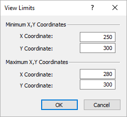
- Select OK.
2.2.2 Add the Opening Section
Now we can add the Opening Section.
- Select Add Opening Section
 on the toolbar or the Boundaries menu.
 - In the Prompt Line at the bottom right of the screen, type t and hit ENTER.

The Enter Coordinates dialog appears. - Enter coordinates as shown below.
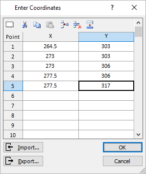
- Select OK.
- In the Prompt, type a and hit Enter .

The Arc Options dialog appears. - Under Arc Defintion Method, select 3 points on arc.
- Under Arc to Polyline Conversion Method, set Number of Segments = 12.
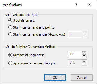
- Select OK.
- In the Prompt, type 271, 320 and hit ENTER.

- In the Prompt, type 264.5, 317 and hit ENTER.

- In the Prompt, type c to close the opening and hit ENTER.

Your screen should look like this.
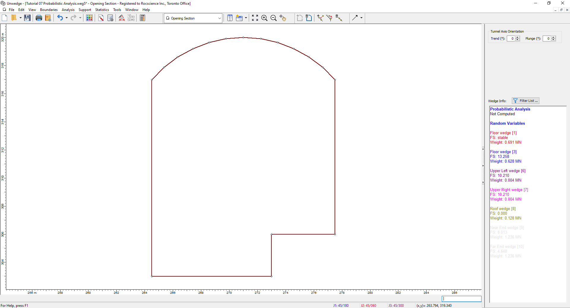
The Opening Section boundary should be automatically zoomed to the center of the view. If it is not, select Zoom All (or press the F2 function key) to zoom the excavation to the center of the view.
3.0 Probabilistic Input Data and Distributions
Now we'll look at the default Joint Orientations and Joint Properties default input data in the Input Data dialog and then define the following as random variables using the Statistics options. All other model input parameters will be assumed to be “exactly” known (i.e., Statistical Distribution = None) and will not be involved in the statistical sampling.
- Joint 1 Orientation
- Joint 2 Orientation
- Joint 3 Orientation
- Phi of Joint Properties 1
3.1 VIEW DEFAULT INPUT DATA
- Select Input Data
 on the toolbar or the Analysis menu.
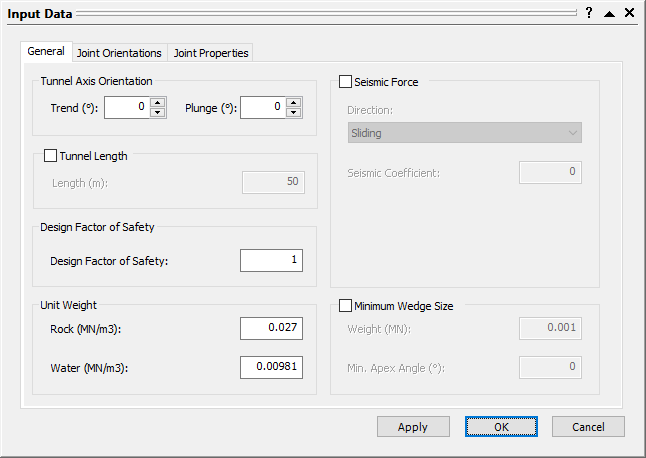
Input Data Dialog - In the General tab, note the Design Factor of Safety.
This option is used in probabilistic analyses for determining the probability of failure and required support pressure. The probability of failure is P(FS < Design FS). - View the default values in the Joint Orientations and Joint Properties tabs but leave them as is.
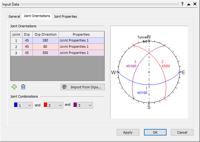
Input Data Dialog 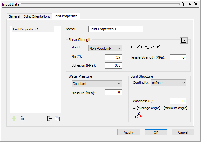
Input Data Dialog - Select Cancel to close the Input Data dialog.
3.2 DEFINE JOINT ORIENTATION VARIABILITY
Now we'll define the variability of the Joint Orientations using the Joint Orientation Statistics dialog. To carry out a Probabilistic Analysis with UnWedge, at least one input parameter must be defined as a random variable.
- Select Joint Orientations
 on the Statistics menu.
The Joint Orientation Statistics dialog appears.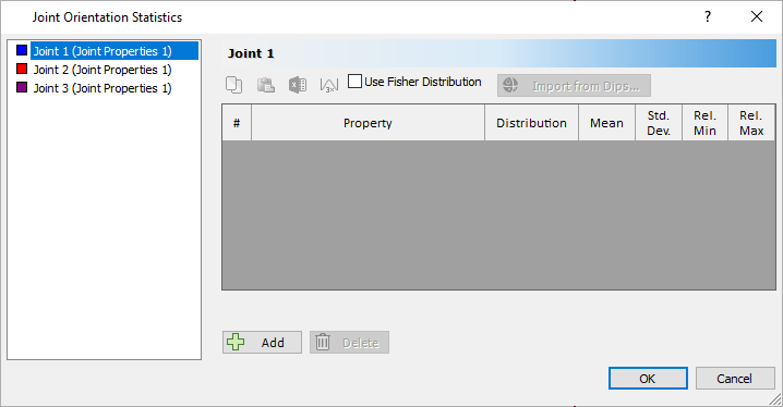
Joint Orientations Statistics Dialog - To define a random variable for the Joint 1 Orientation, click on Joint 1 (Joint Properties 1) on the left.There are TWO methods of defining the variability of joint orientation in an UnWedge Probabilistic Analysis:
- Orientation Definition Method = Dip / Dip Direction
- Orientation Definition Method = Fisher Distribution
With the Dip / Dip Direction method, the Dip and Dip Direction are treated as independent random variables (i.e., you can define different statistical distributions for each one).
- Click the Add
 button in the Joint Orientations dialog.
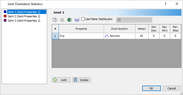
Joint Orientations Statistics Dialog
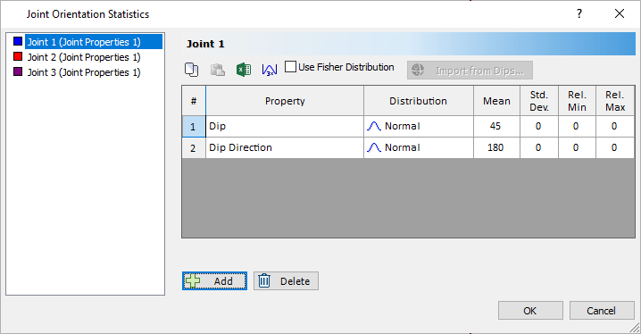
Notice that Dip has been added to the list of Distributions and that it has a Normal Distribution. By clicking on the Distribution dropdown, you can select various other distribution types. - Click the Add button again to add Dip Direction to the list as another random variable.
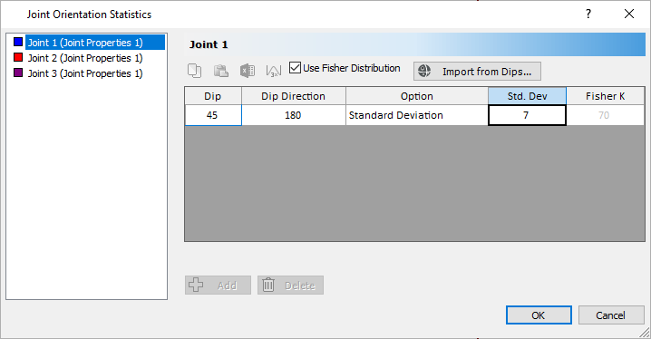
Joint Orientations Statistics Dialog - Check the Use Fisher Distribution checkbox.
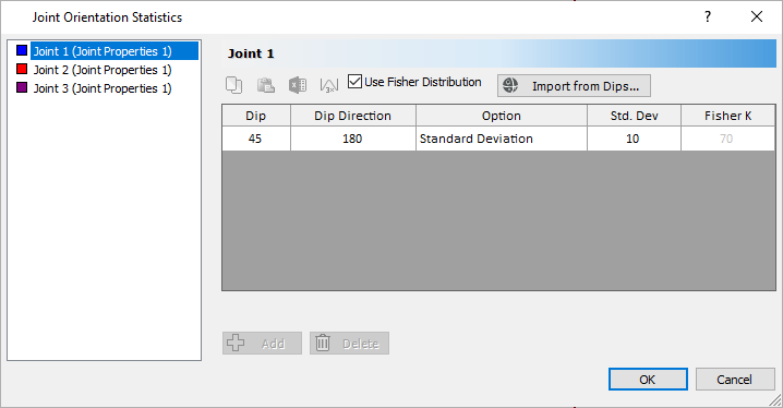
Joint Orientation Statistics dialog
The Fisher Distribution method generates a symmetric, three-dimensional distribution of orientations around the mean plane orientation. Only a single standard deviation is required. In general, a Fisher Distribution is recommended for generating random joint plane orientations because it provides more predictable orientation distributions and lessens the chance of input data errors. - Notice our previous Dip / Dip Direction definitions are now overwritten.
- Set the Standard Deviation = 7.
Joint Orientations Statistics Dialog - Repeat the steps for Joint 2 with a Standard Deviation = 7, and Joint 3 with a Standard Deviation = 10.
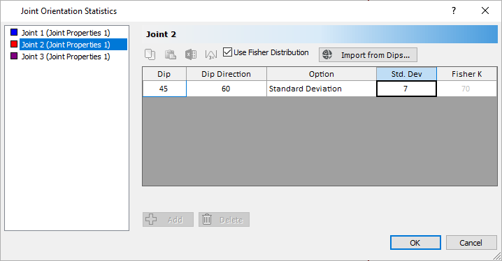
Joint Orientations Statistics Dialog 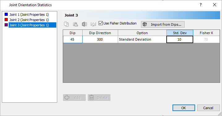
Joint Orientations Statistics Dialog - Select OK.
3.3 DEFINE JOINT PROPERTIES VARIABILITY
We will now define Phi, the angle of internal friction, for Joint Properties 1 as a random variable.
- Select Joint Properties
 on the Statistics menu.
The Joint Properties Statistics dialog appears.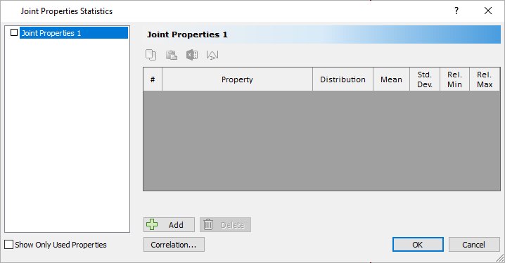
Joint Properties Statistics Dialog
Because all of our joints have the same properties, Joint Properties 1 is the only property on the left of the dialog. - Click the Add button.
The Phi Property is added to the list.
If you click on the Property dropdown, you can see all the other properties you can assign distributions to. - Leave Distribution = Normal.
- Set Std. Dev. = 5 and Rel. Min = 15 and Rel. Max = 15 .
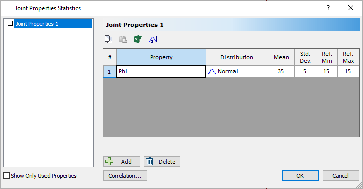
Joint Properties Statistics Dialog - Select OK.
4.0 Compute
We are now ready to compute.
- Select Compute
 on the toolbar or the Analysis menu.
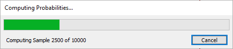
Using the Latin Hypercube sampling method, UnWedge generates 10,000 random input data samples for each random variable using the specified statistical distributions, and computes the probabilistic output for 10,000 possible wedge arrangements.
The calculation may take a few minutes. The progress of the calculation is indicated in the dialog.
5.0 Probabilistic Analysis Results
5.1 PROBABILITY VIEW
The results of the analysis can be studied in the Probability View.
- Select Probability View
 in the View dropdown on the toolbar or on the View > Select View menu.
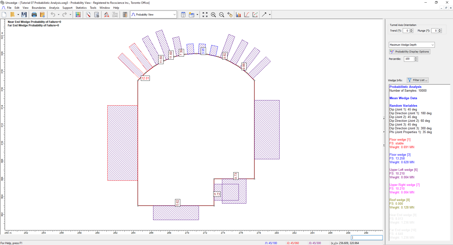
From the dropdown at the top of the Sidebar, we can see that the values in the Wedge Info panel represent the Maximum Support Pressure.
It is important to understand the significance of this cross-section. Due to the variability in our input data, 10,000 different wedge arrangements have been computed. Support Pressure is calculated for each segment from the 10,000 trials and the 10,000 possible wedges that may span this segment. The maximum of these 10,000 possible values is represented by the number displayed on the segment.
You can also use the Percentile option in the Sidebar to adjust which value of Support Pressure to show. The default Percentile is 100%, which is the maximum of all support pressure values computed for a particular segment. However, if you wanted to show the 95th percentile, where 95 percent of all support pressure values for this segment lie below this value, this is possible as well. Take note that Maximum Support Pressure and all probabilistic output is a function of location on the tunnel perimeter.
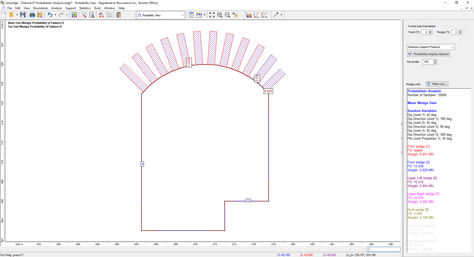
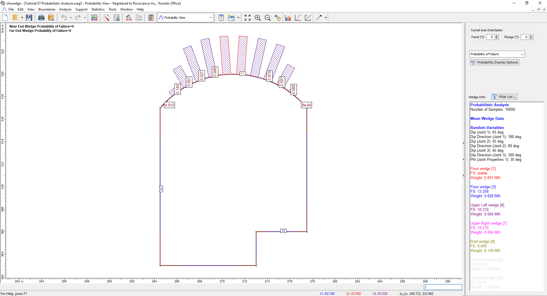
- In the Sidebar dropdown, select Probability of Failure from the Sidebar.
Your screen should look as follows:

Notes:
- Because the wedges on the sides of the tunnel have Factors of Safety greater than our Design Factor of Safety = 1, their Probability of Failure is zero.
- Similarly, because the Roof wedge (8) had a Factor of Safety of 0.000, its Probability of Failure is 1.000.
5.2 WEDGE DISPLAY
- Select 3D Wedge View
 from the View dropdown on the toolbar.
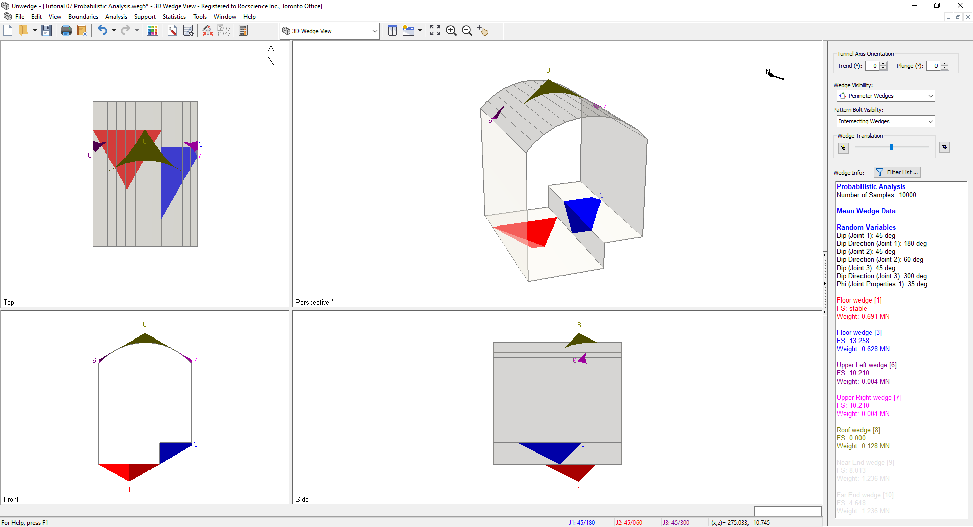
The wedges initially displayed after a Probabilistic Analysis are based on the mean input values and are referred to as Mean Wedges. They will appear exactly the same as ones based on Deterministic Input Data and have the same Factors of Safety, as shown in the Sidebar.
5.3 HISTOGRAMS
To plot histograms of results after a Probabilistic Analysis:
- Select Plot Histogram
 on the Statistics menu.
The Histogram Plot Parameters dialog appears. - Select Factor of Safety in from the Data Type dropdown.
- Leave Location as Multiple Segments.
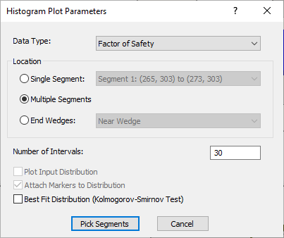
- Click Pick Segments.
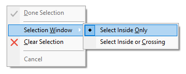
The cursor turns into a selection box. - Right-click on the screen and select Selection Window > Select Inside Only.
- Left-click and, keeping the button pressed, drag a box over just the roof section as shown.
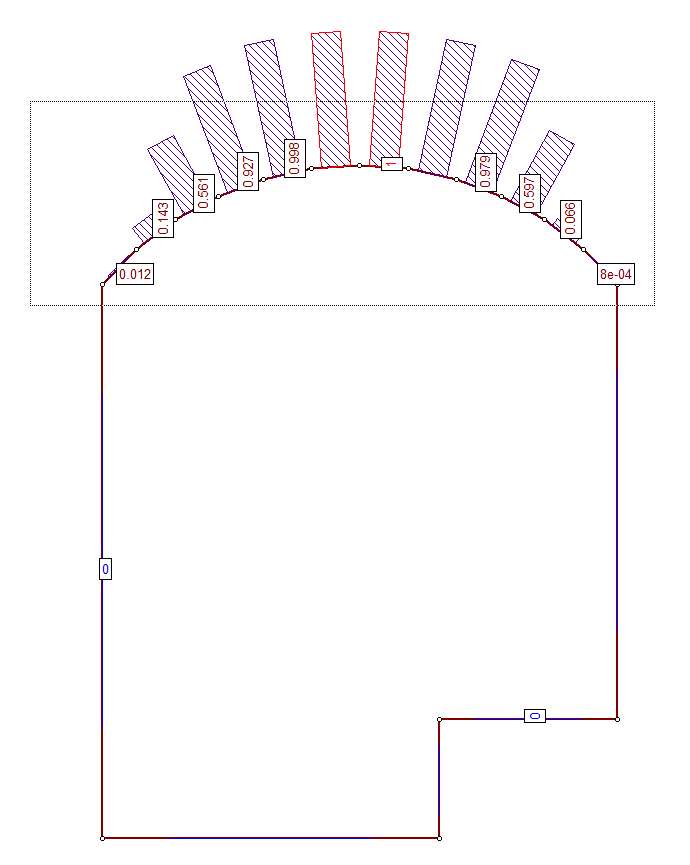
Roof Section View - Release the mouse button and press ENTER.
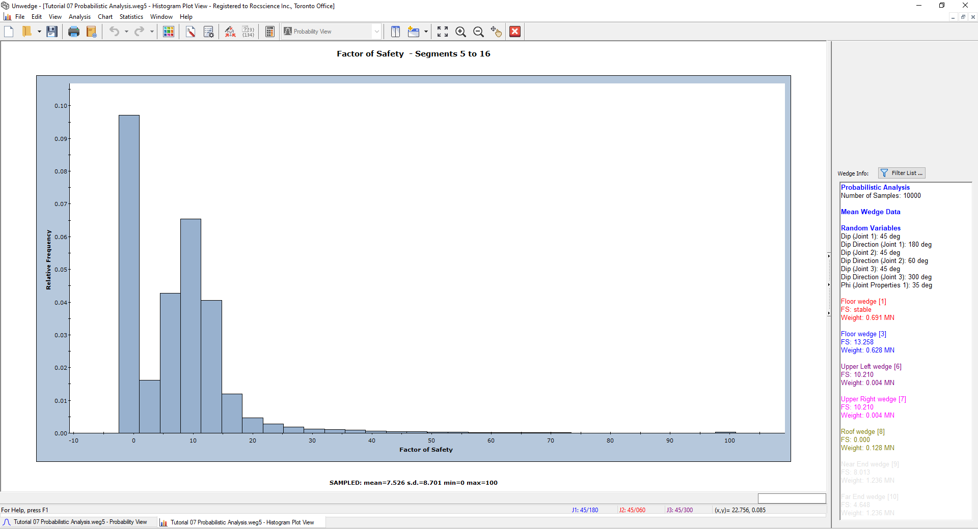
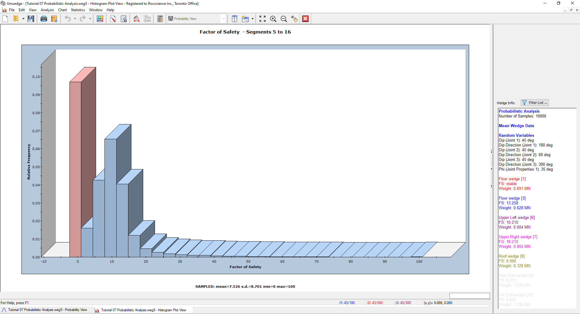
The resulting histogram represents the distribution of Factor of Safety for all valid wedges generated by the random sampling of the Input Data, for all segments comprising the roof of the excavation.
To view Failed Wedges:
- Right-click on the Histogram and select 3D Histogram from the popup menu.
- Right-click again and select Show Failed Wedges.
This option shows the failed wedges (FS < Design FS) along with the safe wedges (FS > Design FS) on the same Histogram. The failed wedges are depicted in red.
5.4 PICKED WEDGE
- Right-click on the Histogram and select 3D Histogram to turn the setting off.
- Select New Window
 on the toolbar or the Window menu.
This option opens a 3D Wedge View and tiles the Histogram with all other open views. - Minimize the Probability View.
- Select Tile Vertically
 from the toolbar such that you see the 3D Wedge View and Histogram side-by-side as shown below.
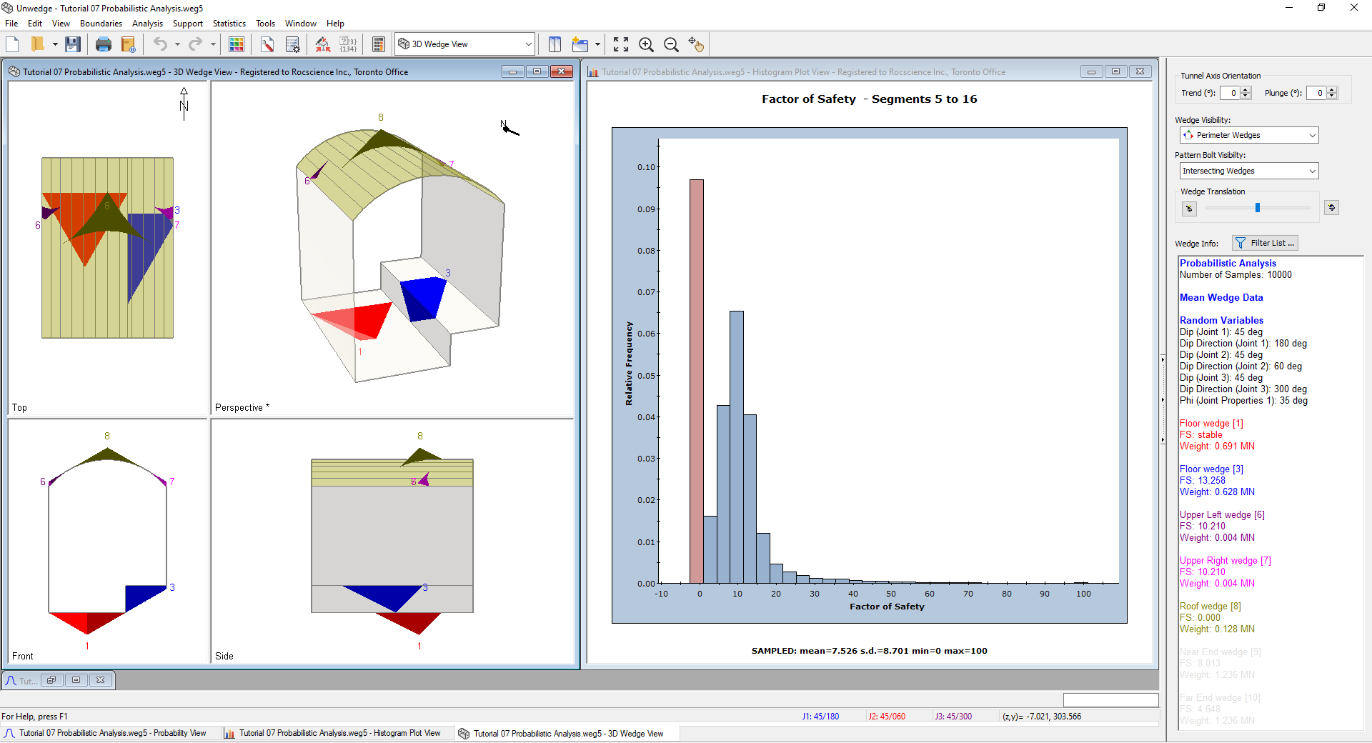
A useful property of Histograms (as well as Cumulative Plots and Scatter Plots) is the following: If you double-click the LEFT mouse button anywhere on the plot, the nearest corresponding wedge is displayed in the 3D Wedge View and results for the wedge are displayed in the Sidebar.
For example:
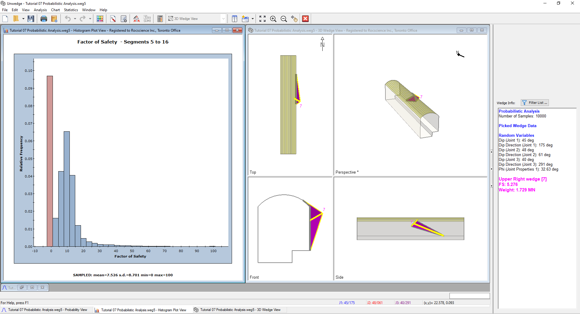
- Double-click on the Histogram somewhere where the Factor of Safety is about 5.
Notice that the wedge in reference is now displayed and has been highlighted. In the Sidebar, the analysis results are updated to display results for the wedge that you are viewing. The wedge has a Factor of Safety of about 5 in the Sidebar, as expected. - Double-click at various points along the Histogram, and notice the different wedges and analysis results that are displayed.
This feature allows you to view any wedge computation generated by the Probabilistic Analysis, corresponding to any point on a Histogram, Cumulative Plot, or Scatter Plot. In addition to the 3D Wedge View, all other applicable views (for example, the Info Viewer and the Stereonet View) are also updated to display data for the currently Picked Wedge.
Notes:
- This feature can be used on Histograms of any statistical data generated by UnWedge, and not just the Factor of Safety Histogram
- This feature also works on Scatter Plots and Cumulative Plots.
To reset the Mean Wedges display:
- Close the Histogram and 3D Wedge View.
- Maximize the Probability View.
- Select View > Show Mean Wedges.
5.5 HISTOGRAMS OF OTHER DATA
In addition to the Factor of Safety, you can also plot Histograms of:
- Other random output variables (e.g., Wedge Weight, Support Pressure)
- Random input variables (i.e., any input data variable that was assigned a statistical distribution)
5.5.1 Other Random Output Variables
- On the Sidebar, change the display to Maximum Wedge Depth.
Again, note that due to the variability in our input data, 10,000 different wedge arrangements have been computed. Wedge Depth is calculated for each segment from the 10,000 trials. The maximum of these values is represented by the number displayed on the segment. It should also be noted that the Wedge Depth discussed here and the Apex Height which can be displayed in the Sidebar are synonymous. - Click on the roof segment on the left (with Maximum Wedge Depth = 12.01).
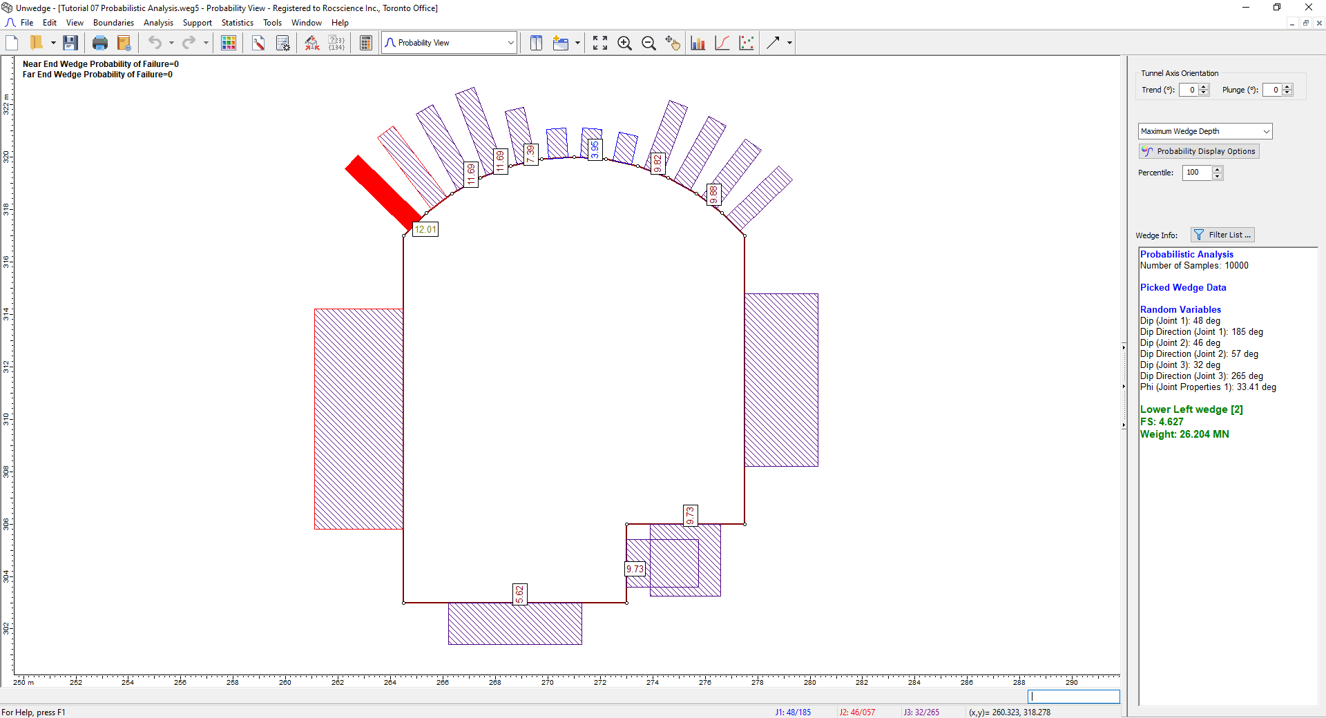
The segment should turn red. - Select Plot Histogram on the toolbar or the Statistics menu.
- In the Histogram Plot Parameters dialog, set Data Type = Wedge Depth
- Ensure Single Segment is selected. Set the Single Segment = Segment 16: (265, 318) to (265, 317).
- Select the Best Fit Distribution checkbox.
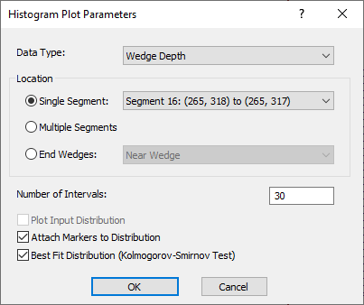
- Select OK.
A histogram of the wedge depth and the best-fit distribution to the data is displayed. - Select the New Window button from the toolbar or the Window menu.
You should now see a tiled view of the Histogram and the 3D Wedge View. - Double-click on the Histogram where the Maximum Wedge Depth is about 12 m.
The wedge will be displayed on the 3D Wedge View, as shown below.
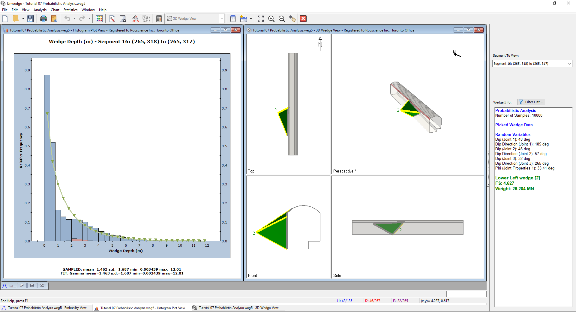
We can now see from the 3D Wedge View that the relatively large Maximum Wedge Depth for this segment and the adjoining segment to the right is due to a side wedge that intersects the upper left corner of the roof.
To reset the Mean Wedge display:
- Close the Wedge Depth Histogram view and the 3D Wedge View.
- Maximize the Probability View.
- Select View > Show Mean Wedges.
5.5.2 Input Random Variables
Now let’s generate a Histogram of an input random variable.
- Select Plot Histogram on the toolbar or the Statistics menu.
- In the Histogram Plot Parameters dialog, set Data Type = Dip (Joint 1).
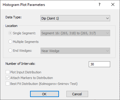
- Select OK.
The Histogram is depicted below.
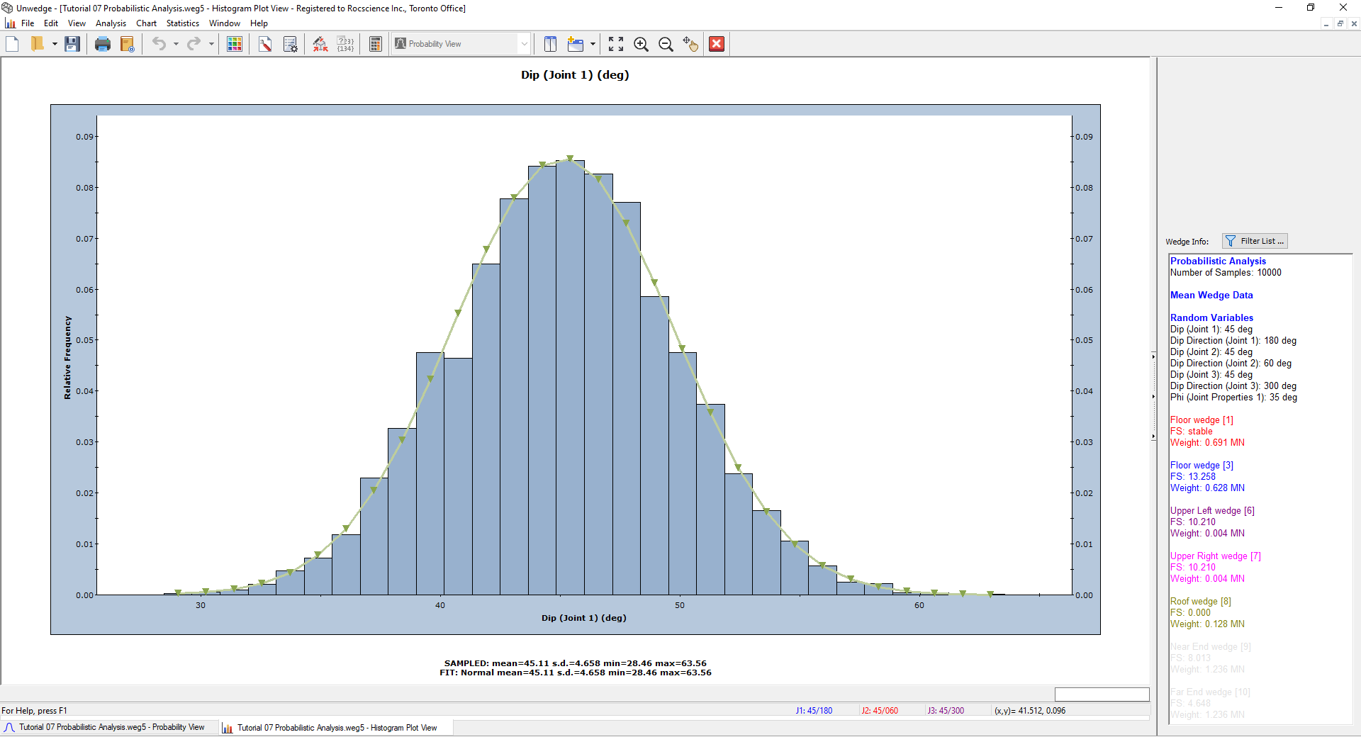
For input random variables, the Input Distribution can be displayed on histograms. However, because the orientation of Joint 1 was generated using a Fisher Distribution, which is three-dimensional, the Input Distribution cannot be displayed on the Histogram, which is a two-dimensional plot of only one component (Dip) of the Joint 1 orientation.
- Return to the Probability View by clicking on the Probability View tab on the bottom left of the screen.
5.6 SCATTER PLOTS
Scatter plots allow you to examine the relationship between any two analysis variables.
To generate a Scatter Plot:
- Select Plot Scatter
 on the toolbar or the Statistics menu.
 - In the Scatter Plot Parameters dialog, select the variables you would like to plot on the X and Y axes. For example, let’s plot the Factor of Safety versus Dip (Joint 1).
- Set X-Axis Dataset = Factor of Safety.
- Set Y-Axis Dataset = Dip (Joint 1).
- Ensure Multiple Segments is selected.
- Select the Show Regression Line option to display the best fit straight line through the data.
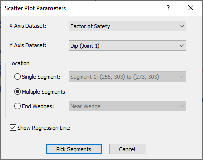
- Click Pick Segments.
- Select all the roof segments using the mouse as before.
- Press ENTER.
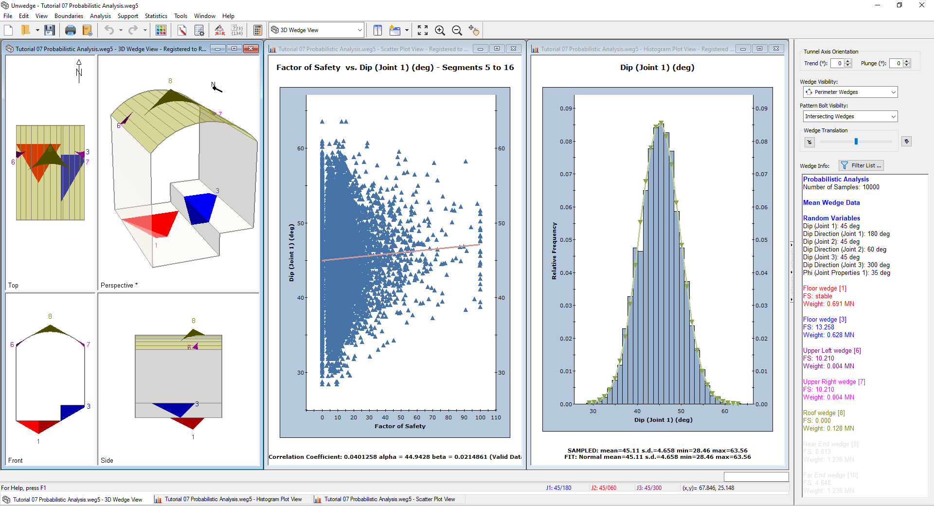
The following scatter plot should appear.
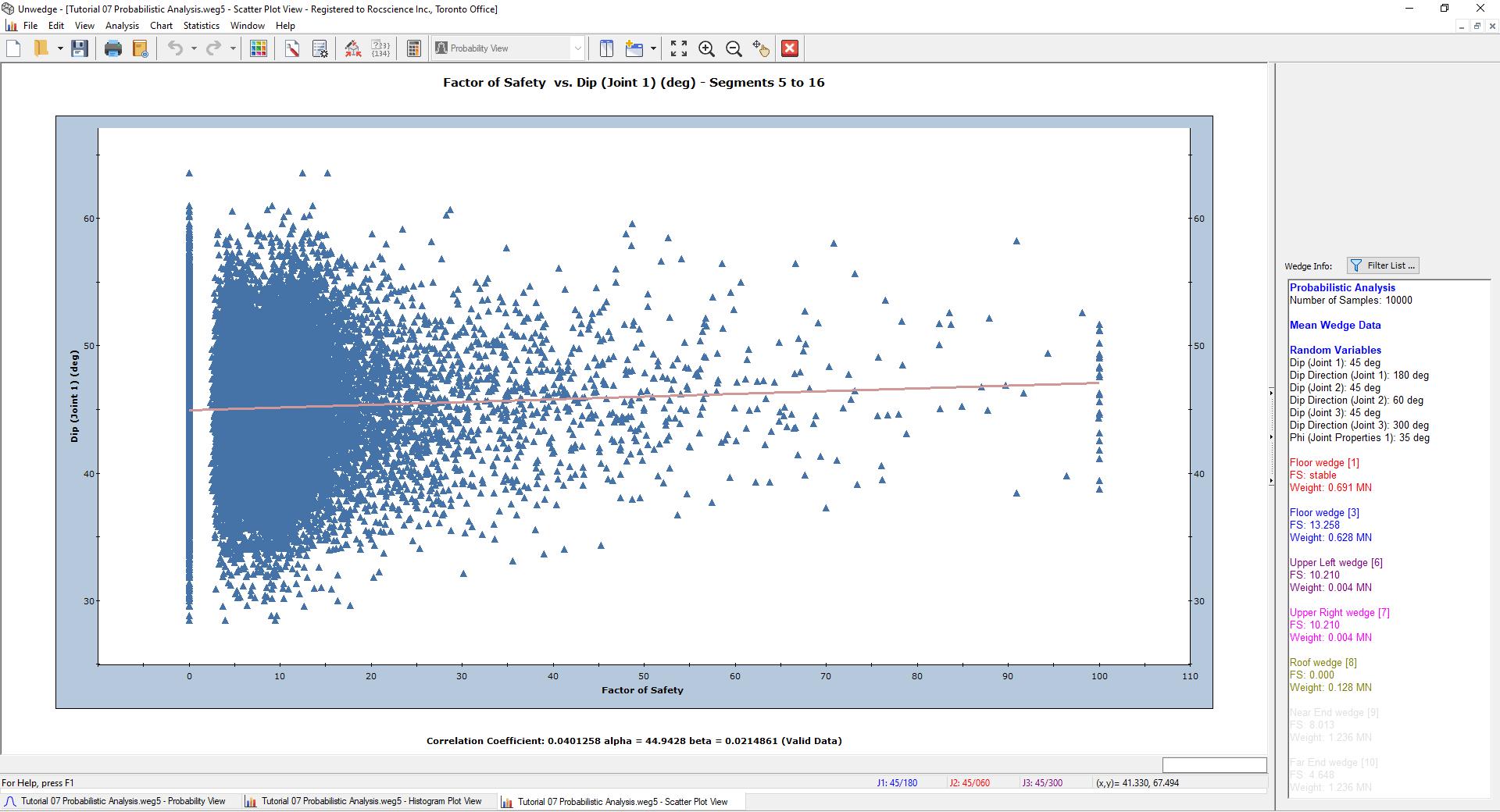
Note the Correlation Coefficient listed at the bottom of the plot, which indicates the degree of correlation between the two variables plotted. The Correlation Coefficient can vary between -1 and 1 where numbers close to zero indicate a poor correlation and numbers close to 1 or -1 indicate a good correlation.
6.0 Compute (Random Sampling)
So far in this tutorial we have used the default Pseudo-Random sampling option. Pseudo-Random sampling allows you to obtain reproducible results for a Probabilistic Analysis by using the same “seed” value to generate random numbers. This is why you can obtain the exact values shown in this tutorial. We will now demonstrate how different outcomes can result from a Probabilistic Analysis by allowing a variable seed value to generate the random input data samples.
Before we start, let’s arrange the views as follows:
- Select the Tile Vertically option from the toolbar or the Window menu to tile all of the open views.
You should have Probability View, Histogram Plot, and Scatter Plot open. - Click on the Probability View and switch to the 3D Wedge View.
You should see the following on your screen.
If your screen does not look similar to the figure (e.g. you have additional views open), then close all views except for the three noted above such that your screen resembles the figure.
To switch to Random Number Generation:
- Select Project Settings on the toolbar or the Analysis menu.
- In the Project Settings dialog, select the Random Numbers tab.
- Change the Random Number Generation method from Pseudo-Random to Random.
 The Random option uses a different seed value to generate random numbers each time you re-run the Probabilistic Analysis. This will result in a different sampling of your input random variables, and different analysis results (e.g., Probability of Failure) each time you re-compute.
 - Select the Sampling tab.
- Decrease the Number of Samples from 10,000 to 1,000 to make the change in results easier to see on the plots.
- Select OK.
- Select Compute on the toolbar.
Notice that the Histogram Plot and Scatter Plot are updated with new results.
UnWedge will only allow the user to select Compute if a change has been made to the input data. In order to see the way that data changes when using Random Number Generation, we want to select Compute repeatedly. To do this:
- Select File > Preferences
 and make sure the Disable compute button when results are up to date option is unchecked.
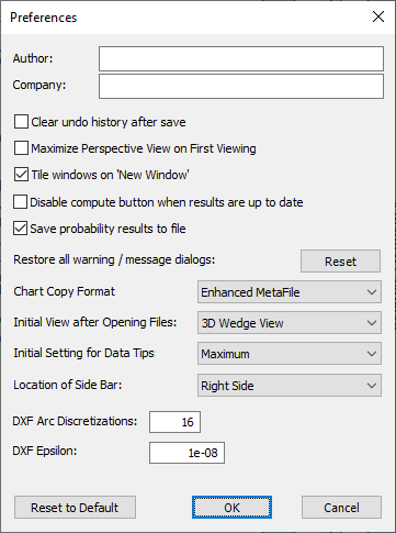
- Select OK.
- Select Compute repeatedly and observe how the windows are updated each time the analysis is re-run.
7.0 References
Bond, A. J. and Harris, A. J., 2008. Decoding Eurocode 7, Taylor & Francis.
British Standards Institution, 2004. Eurocode 7: Geotechnical design – Part 1: General rules, BS EN 1997-1, London, UK.
Smith, 2006. Smith’s Elements of Soil Mechanics, 8th Edition, Blackwell Publishing.
That concludes the UnWedge Probabilistic Analysis Tutorial.