Joint Slope Stability Analysis Using SSR
1.0 Introduction
This tutorial introduces how to add a joint surface onto a slope and conduct slope stability analysis using the Shear Strength Reduction (SSR) method in RS3.
All tutorial files installed with RS3 can be accessed by selecting File > Recent > Tutorials folder from the RS3 main menu. The initial file of the tutorial can be found in Joint slope stability SSR - starting file.rs3v3 and the finished tutorial can be found in the Joint slope stability SSR - final.rs3v3 file.
2.0 Starting the Model
- Select File > Recent > Tutorials Folder.
- Open Joint slope stability SSR - starting file.rs3v3.
- Open the Project Settings dialog by selecting Analysis > Project Settings

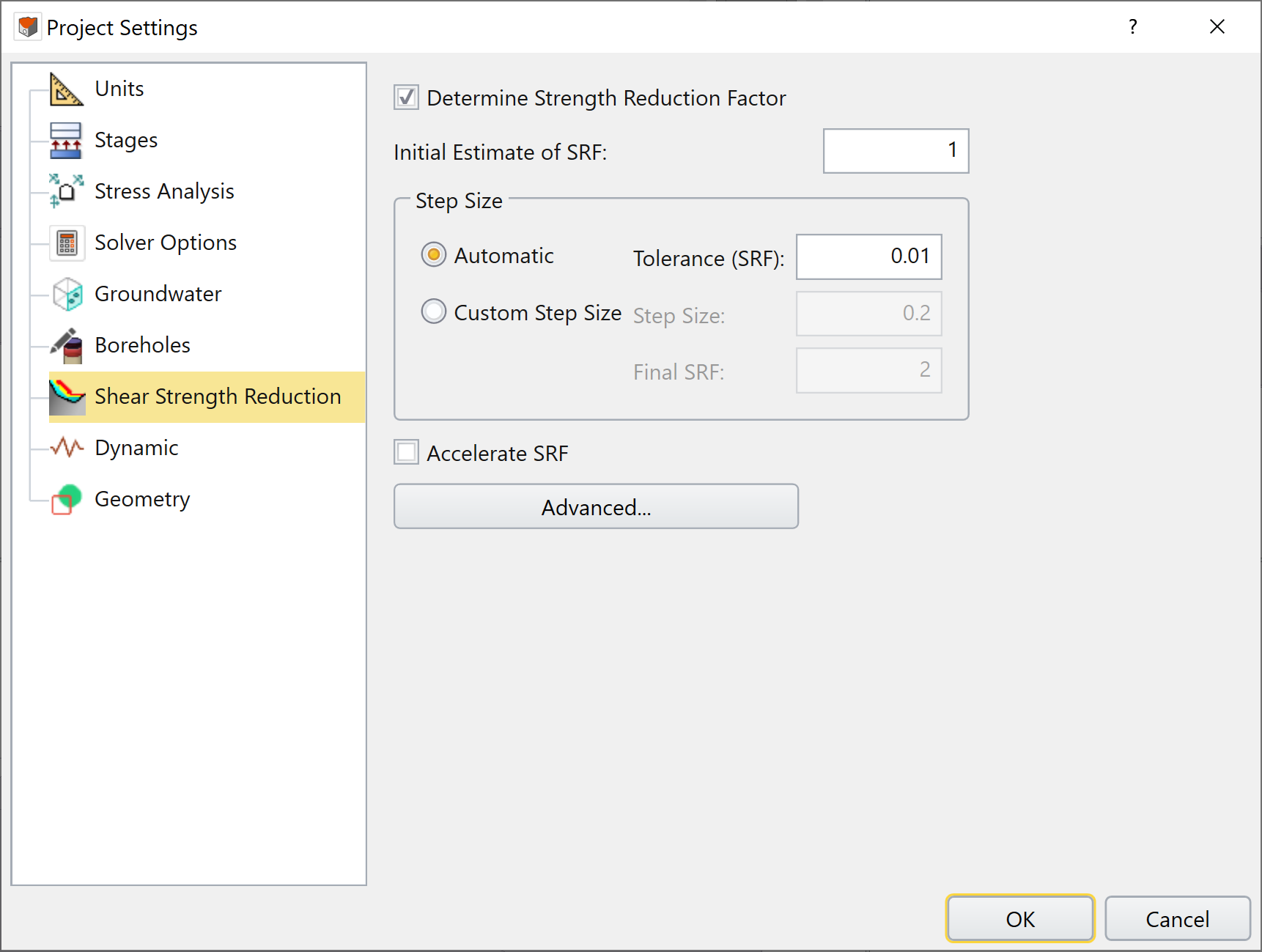
- Select the Shear Strength Reduction tab. Make sure the option 'Determine Strength Reduction Factor' is enabled and the inputs as:
- Initial Estimate of SRF = 1,
- Step Size of Automatic Selected, and
- Tolerance (SRF) = 0.01.
- Click OK to close the dialog.
3.0 Adding a Joint Surface
- Ensure the Geology workflow tab is selected

Before we begin with creating the joint surface, we will first select the thin extruded slope volume and set it as an external geometry.
- Select the Volume 0 entity in the Visibility Tree, then select Geometry > Set as External.

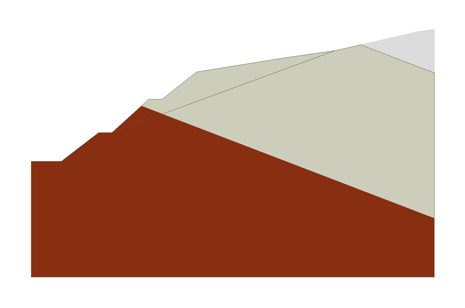
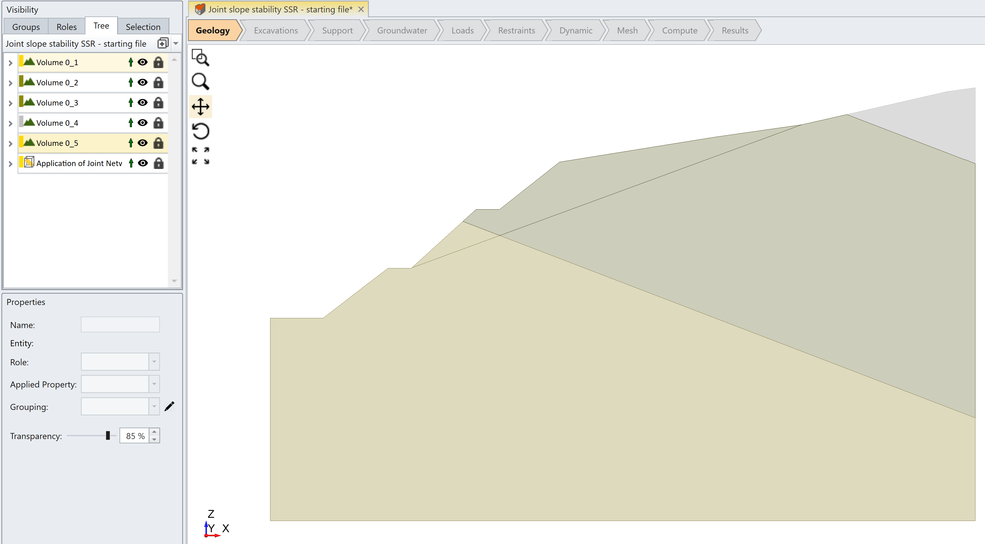
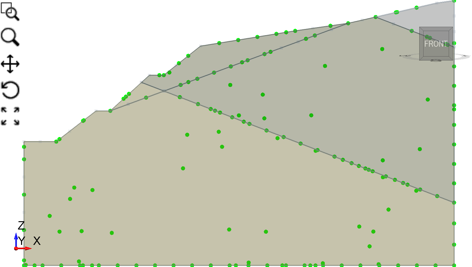
- Now select the 'Application of Joint Networks (initial)_JOINT_BOTH_CLOSED' plane entity in the Visibility Tree. With the plane entity selected, your model should look as follows:

- Select: Materials > Joints > Add Joint Surface.

- In the Add Joint Surface dialog, keep all default settings and click OK. The plane entity has been converted to a joint surface.
Now we will use the Divide All Geometry option to create external volumes.
- Select: Geometry > 3D Boolean > Divide All Geometry
- Keep all settings as default as shown:

- Click OK. The external volumes are now defined.
4.0 Assigning Materials
You will see multiple volumes in the Visibility Tree. We want to assign each layer of soil to Zone I, Zone II and Zone III.
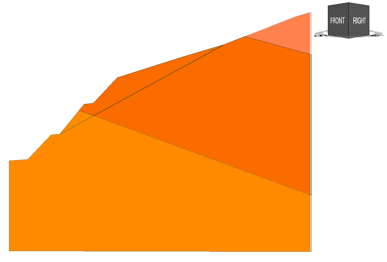
- Select the Volume 0 entity in the Visibility Pane that corresponds to the top right volume of the model in the ZX plane viewport as shown below.
- In the Properties Pane, change the Applied Property to Zone I.

- Hold CTRL and select the two volumes beneath Zone I as shown below and change the Applied Property to Zone II.

- Hold CTRL and select the bottom two volumes of the model and assign change the Applied Property to Zone III.
- The soil layers should be assigned as follows.
5.0 Restraints
- Select the Restraints workflow tab

- Select the Faces Selection option
 from the toolbar. While holding CTRL, select (left-click) the front (XZ) faces of the model as shown below.
 - Select: Restraints > Add Restraints / Displacement > Restrain Y.
- In the Add Restraint dialog, click OK. Now you will see the assigned restraints on the front of the model as shown below.
Do the same for the back face (XZ plane) of the model by rotating the 3D viewcube.
- Now select the left and right side (YZ) faces of the model as shown below:
- Assign XY restraints by selecting Restraints > Add Restraints/Displacements > Restrain XY.
- In the Add Restraint dialog, click OK.
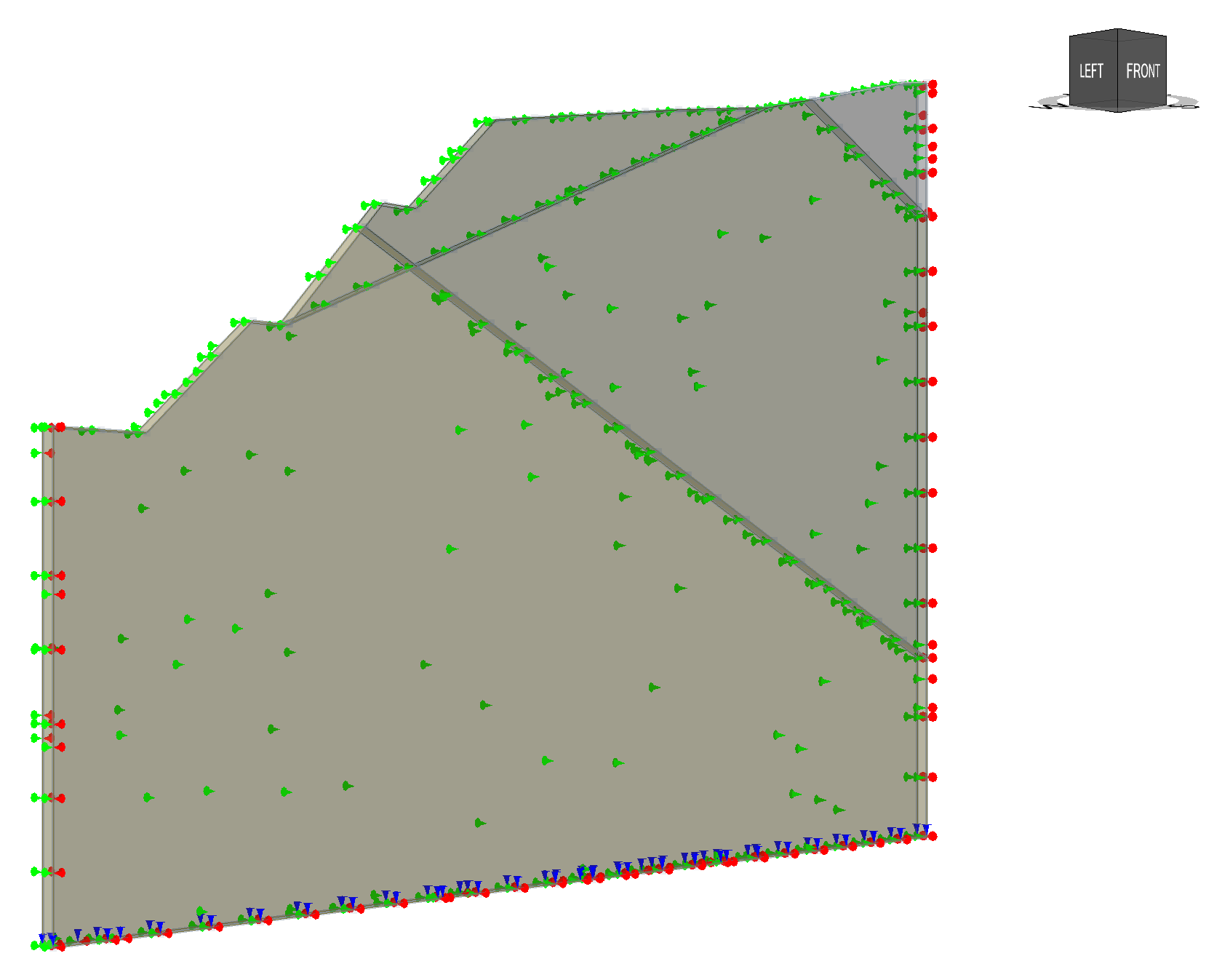
- Now, select the bottom face and assign restraint XYZ by selecting Restraints > Add Restraints/Displacements > Restraint XYZ. In the Add Restraint dialog, click OK. Then, you will see the following restraints as shown below.
6.0 Mesh
- Next, we move to the Mesh workflow tab

Here we may specify the mesh type and discretization density for our model.
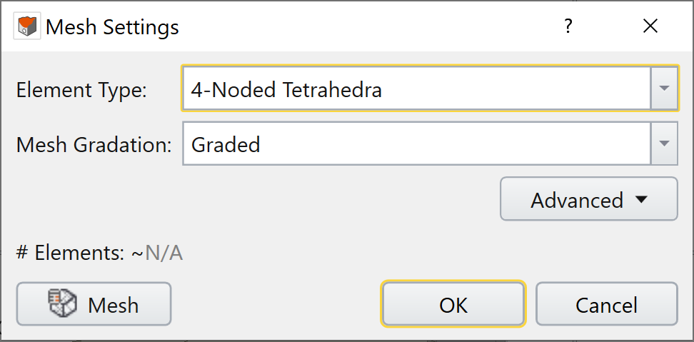
- Select: Mesh > Mesh Settings
- Use the following settings:
- Element Type = 4-Noded Tetrahedra,
- Mesh Gradation = Graded.
- Select Mesh to mesh the model.
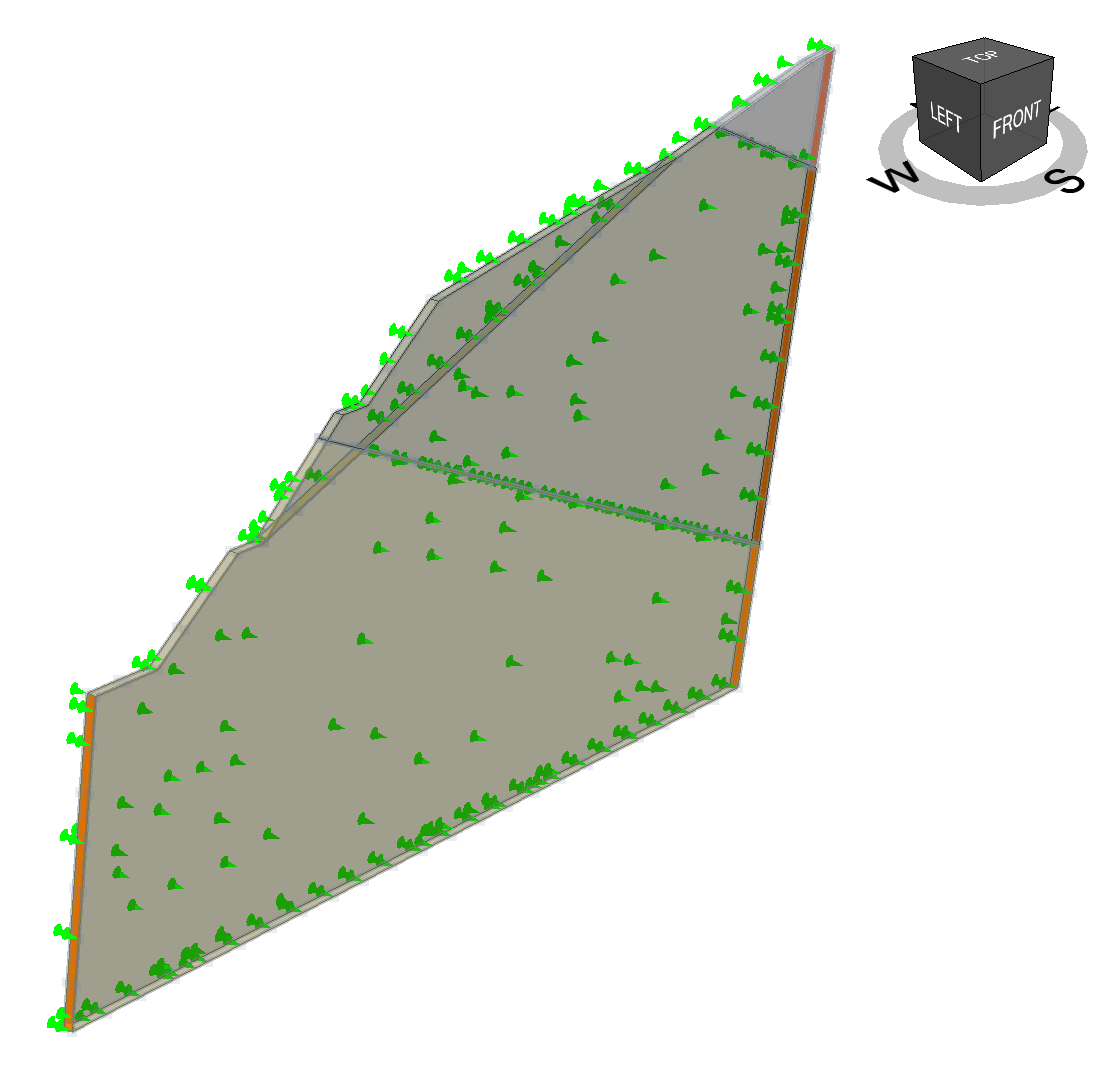
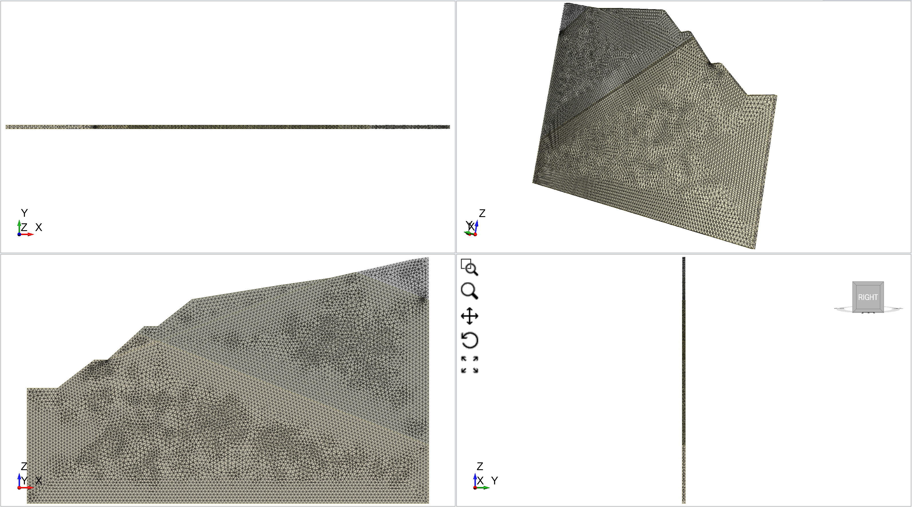
The mesh is now generated, your model should look like the one below.
Now we will compute the model.
7.0 Compute
- Next, we move to the Compute workflow tab

- From this tab, we can compute the results of our model. First, save your model: File > Save As.
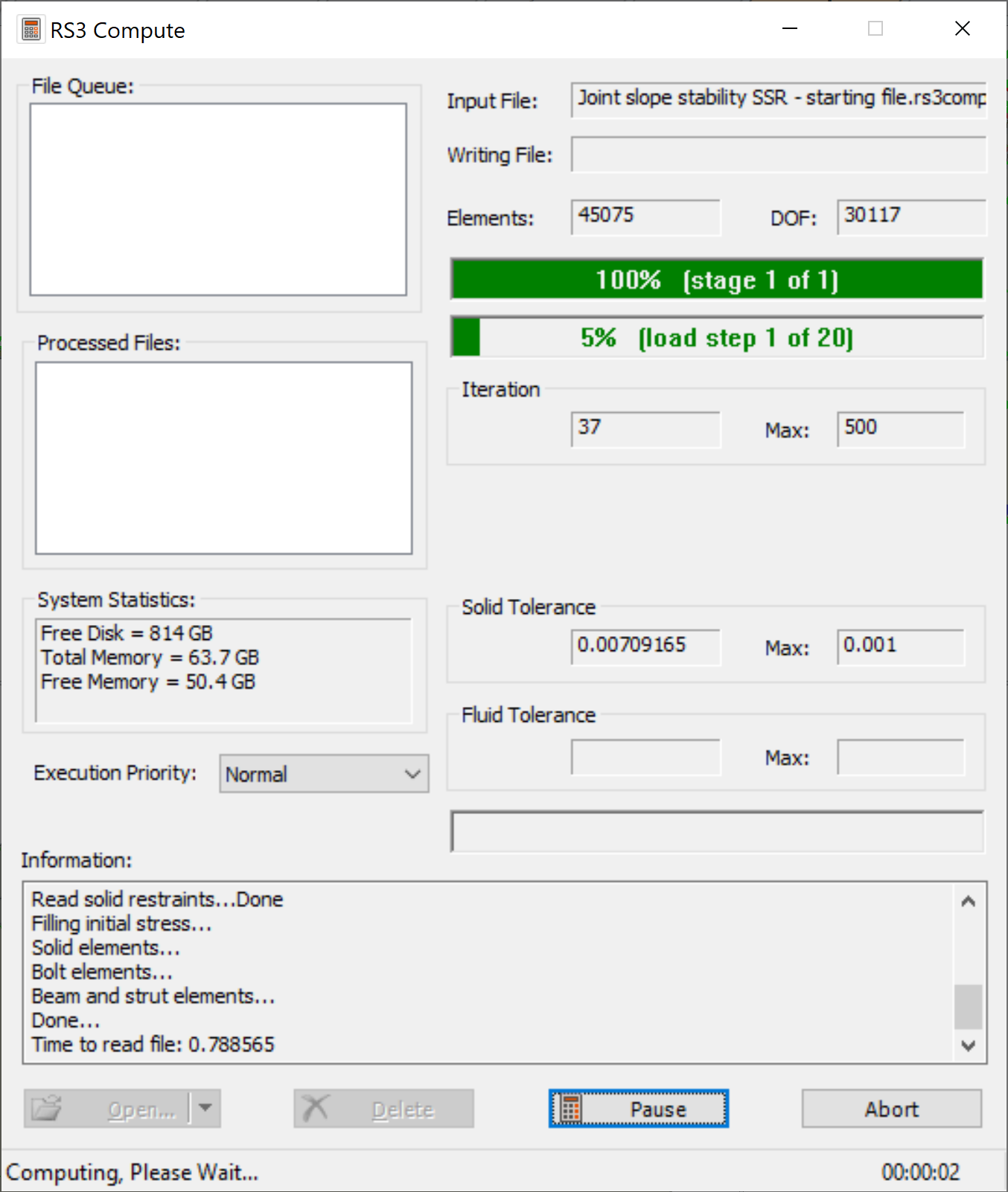
- Use the Save As dialog to save the file. You are now ready to compute the results. SSR analysis requires multiple iterations to locate the Critical SRF which increases the computation time. Computation should take about 20 minutes depending on your computer specifications.
- Select: Compute > Compute

8.0 Results
- Next, once the computation is complete we move to Results workflow tab

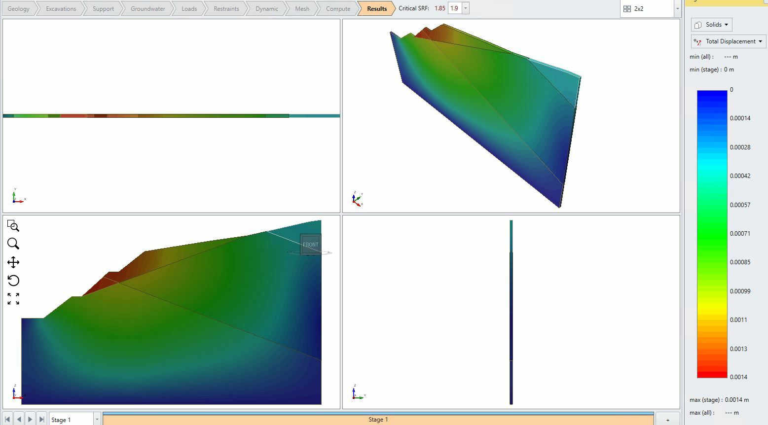
Right beside the Results tab, you will see the Critical SRF value of 1.85 when the model fails.
- In the legend, change Data Type to Total Displacement and under the SRF drop-down menu change it to 1.9. The SRF text colour indicates the model has failed if it's red.
- Select: Interpret > Show Exterior Contour

As shown below, the critical zone of failure occurs in the volume of material that is sliding along the joint surface.
This concludes the tutorial on jointed slope stability analysis using SSR in RS3