12 - Fragmentation

This tutorial introduces the Fragmentation analysis in RocFall2. Fragmentation in rockfall occurs on impacts and is a complex phenomenon dependent on a number of material, discontinuity, and kinematic factors. An overview of the Fragmentation analysis, including assumptions and limitations, can be found in the Fragmentation Overview help topic.

Topics Covered in this Tutorial:

• Creating a fragmentation analysis
• Material characterizations
• Results interpretation
• Effects of fragmentation on protection design

Finished Product

The finished product of this tutorial can be found in the Tutorial 12 - Fragmentation data file. All tutorial files installed with RocFall2 can be accessed by selecting File > Recent Folders > Tutorials Folder from the RocFall2 main menu.

1.0 Introduction

A stochastic rockfall analysis in RocFall2 may be conducted with or without considering the effects of fragmentation. To consider the effects of fragmentation, the analysis method must be Lump Mass and material characterization must be provided for the slope materials and falling rock (seeder) materials. This is because the Guccione et al. (2025) fragmentation model is an empirical formulation based on laboratory fragmentation of intact, spherical rock-like specimens with simplified kinematics. The effects of discontinuities on fragmentation and rigid body dynamics considering rock shape are not considered in this fragmentation formulation.

2.0 Model

Let’s start by opening the initial file for this tutorial.

1. Select File > Recent Folders > Tutorials Folder and open the Tutorial 12 initial file.

You should see the following model:

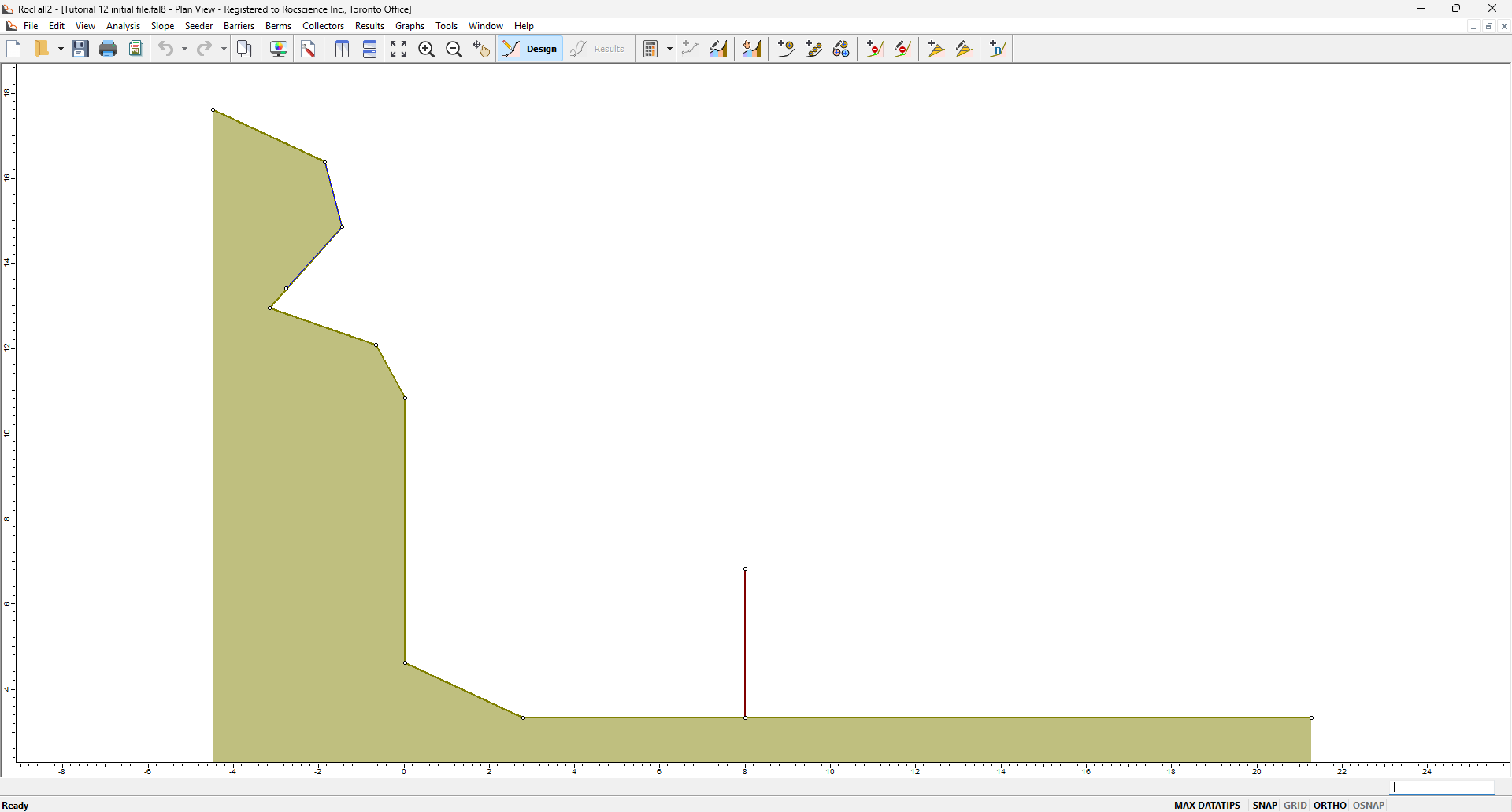
A slope geometry and a line seeder have already been defined. A collector is also installed, where it can collect rockfall data at that location. We still need to set up the Fragmentation analysis and input relevant material characterization parameters for the slope and seeder.

2.1 Project Settings

The Project Settings dialog is used to configure the main analysis parameters of the model, including those for the fragmentation analysis.

1. Select Analysis > Project Settings in the menu or select Project Settings in the toolbar.
2. In the General tab, ensure the Analysis Method is selected as Lump Mass.
3. Select the Fragmentation check box. Notice that Consider rotational velocity becomes disabled for fragmentation analysis. This is because the Guccione et al. (2025) fragmentation model uses simplified kinematics and does not consider rock rotation.
   
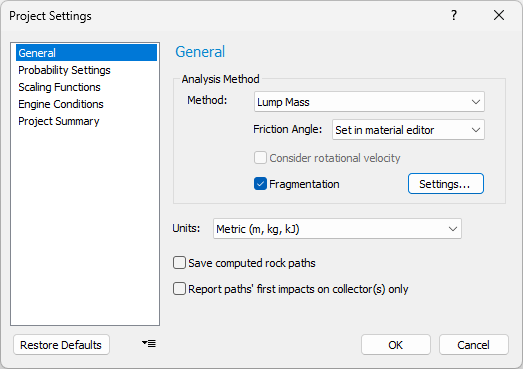
4. Click OK.

2.2 Slope Material Characterization for Fragmentation Analysis

Slope material parameters for fragmentation analysis can be found in the Slope Material Library. The tutorial slope material is Bedrock Outcrops, so we need to further characterize the Bedrock Outcrops for fragmentation analysis.

1. Select Slope > Slope Material Library in the menu or select Slope Material Library in the toolbar.
2. Select the Bedrock Outcrops material and click on the Fragmentation tab. Note that the Fragmentation tab is only available for input when fragmentation analysis is enabled in Project Settings.
3. Use an Ei secant (intact secant modulus from unconfined compressive testing) of 11700 MPa.
   
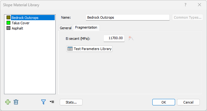
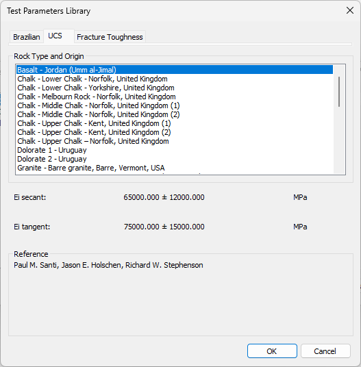
4. For reference values of Ei secant, click Test Parameters Library. The Test Parameters Library contains reference parameter values of the laboratory tests needed to characterize the slope and seeder for fragmentation analysis.
   
   
5. We are not using the Test Parameters Library in this tutorial, so click Cancel to exit the Test Parameters Library.
6. Click OK to accept the Ei secant input and to exit the Slope Material Library dialog.

2.3 Seeder Properties and Material Characterization for Fragmentation Analysis

Seeder material characterization for fragmentation analysis can be found in the Rock Type Library. Let’s view the properties of the line seeder and assign fragmentation material properties to the seeder rock type.

1. Right-click on the line seeder and select Seeder Properties (or select Seeder > Define Seeder Properties and view Seeder 1). 100 rocks are seeded in the analysis and all have Group 1 Rock Type. The rock initial velocities are zero, indicative of a freefall condition.
   
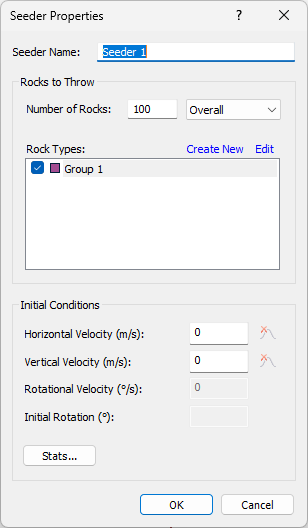
2. In the Seeder Properties dialog of Seeder 1, click Edit to open the Rock Type Library.
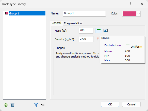
3. Select Group 1. Notice a Uniform distribution is assigned to the rock mass, ranging from 100 kg to 300 kg.
   
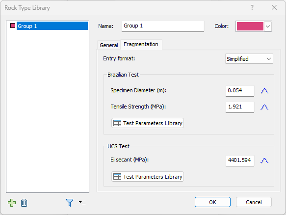
4. For Group 1, select the Fragmentation tab. Note that the Fragmentation tab is only available for input when fragmentation analysis is enabled in Project Settings.
5. Use the default values. However, note that users may access the Test Parameters Library, which contains reference parameter values of the required laboratory tests.



6. Click OK to accept the default values and to exit the Rock Type Library.
7. Click OK again to exit the Seeder Properties dialog.

3.0 Fragmentation Results

Compute to view the resulting rock paths.

1. Select Analysis > Compute in the menu or click Compute in the toolbar.

You should see the following rock paths:

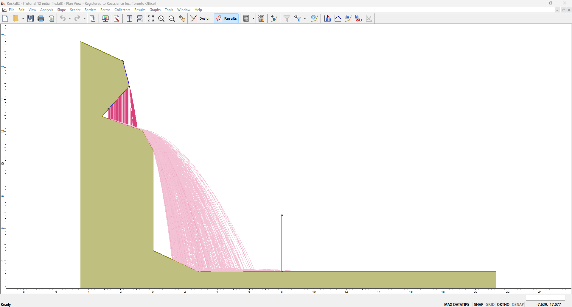
Note that results viewing is always done in Results mode and not in Design mode.

3.1 Collector Data

Let’s first review rockfall data on the collector.

1. Right-click on the collector and select Display Hits. The Number of Hits is 143, which is greater than the 100 rocks assigned to the line seeder. This means that fragmentation occurred for a number of seeded rocks and/or occurred more than once for some rock paths.
2. Right-click on the collector again and select Graph Collector Data (or select Graphs > Graph Barriers and Collectors and choose Collector 1). For the Data to Plot select Block Mass and for the Graph Type select Histogram Plot. Click Graph to get the following:

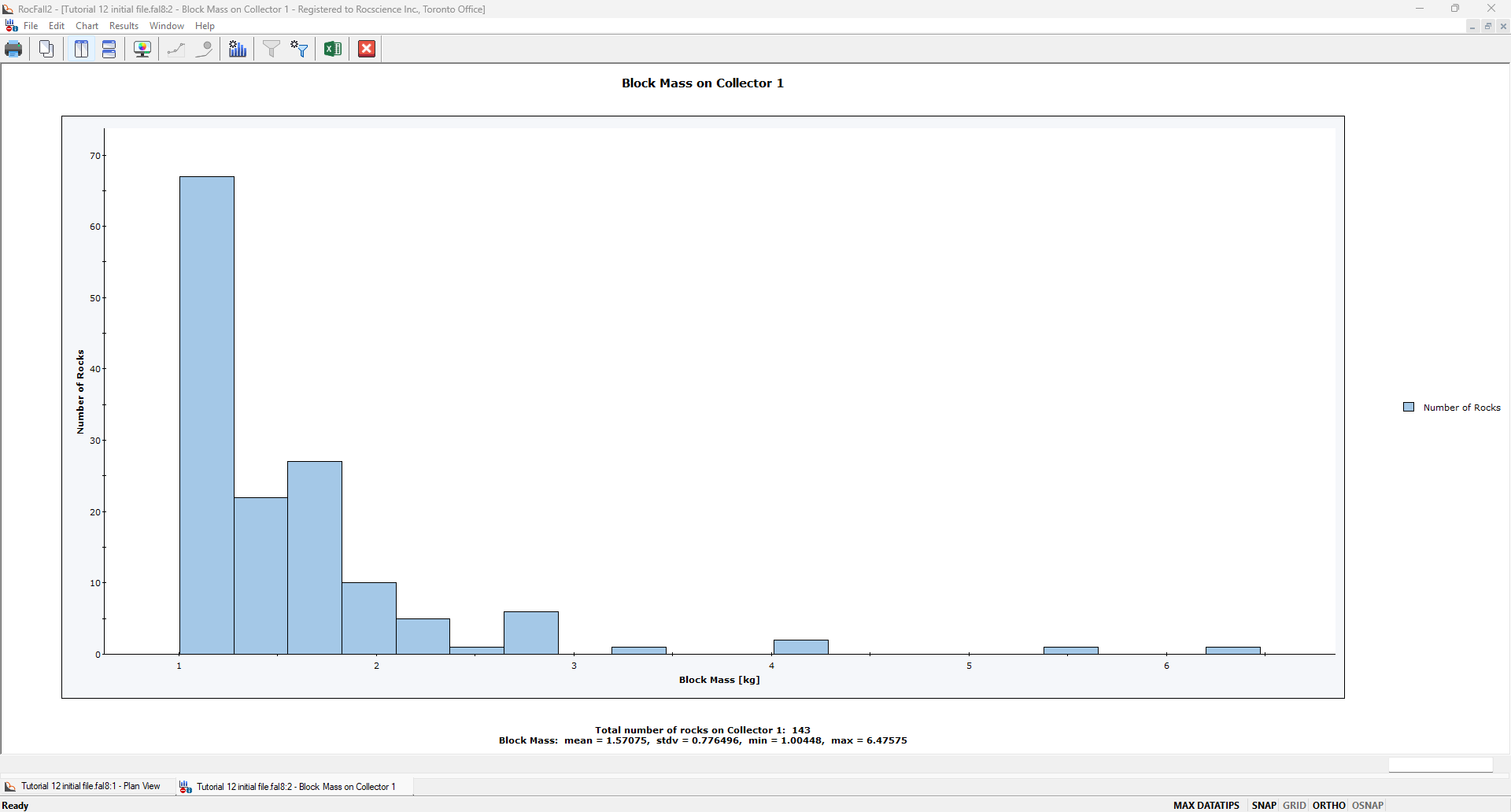
The block mass histogram shows that the rocks hitting the collector are mainly fragments with much smaller masses than those originally assigned to the line seeder. The mean block mass on the collector is approximately 1.6 kg, whereas the seeder was assigned a mass range of 100 kg to 300 kg.

The implication is that a protection system installed at the same location would be designed for smaller rock sizes but potentially a greater frequency of impacts if fragmentation were accounted for in the rockfall analysis.

3.2 Fragmentation vs. No Fragmentation

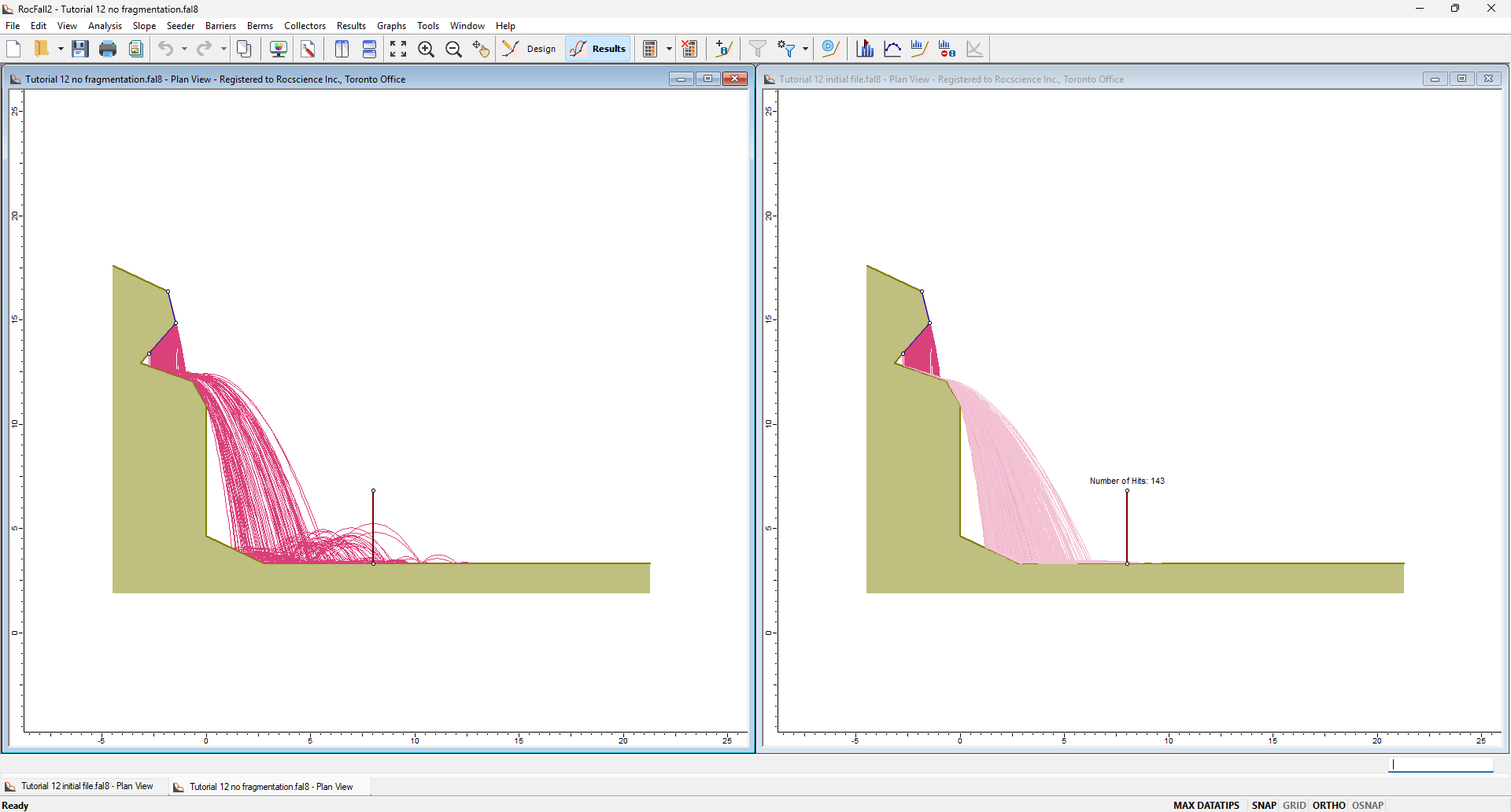
Let’s compare the analysis with and without fragmentation. The same analysis without fragmentation can be viewed in the following model file:

1. Select File > Recent Folders > Tutorials Folder and open the Tutorial 12 no fragmentation file.
2. Select Analysis > Compute

A comparison of the two models shows that fragmentation had a significant effect on energy loss, which can be interpreted using the following tools:

3. Select Window > Tile Vertically. The following shows rock paths for analysis without fragmentation on the left and with fragmentation on the right. It’s obvious that rock path heights are smaller for the case on the right (with fragmentation).
   
4. For each model, select Graphs > Graph Data on Slope . As the Data to Plot select Total Kinetic Energy, and check Max, Mean, 1^st Percentile (95%), and 2^nd Percentile (68%). Select Plot Data.
5. Minimize the model windows to view only the two graphs. Select Window > Tile Vertically. This should vertically tile the two graph views.

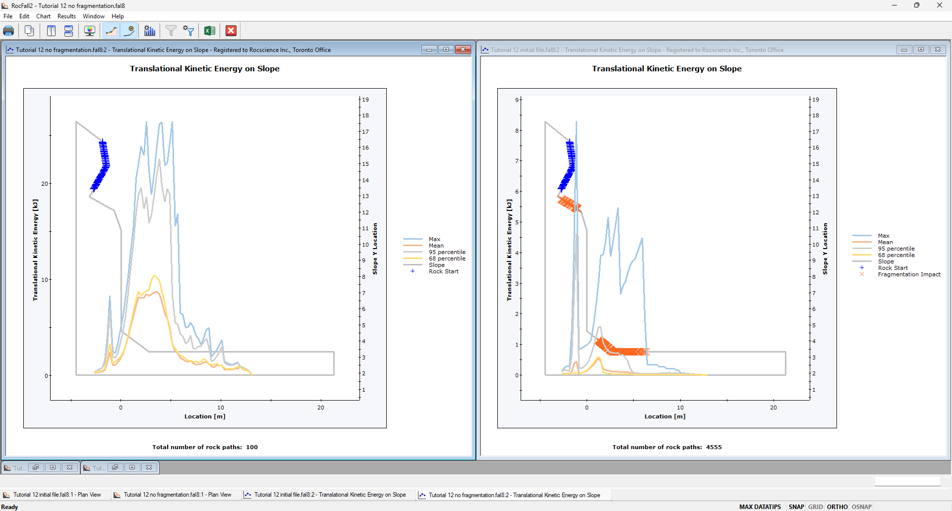
The total kinetic energy profiles for the case on the right (with fragmentation) are much smaller than for the case on the left (without fragmentation). Also notice the orange markers indicating the locations where fragmentation occurred, and a significant drop in the total kinetic energy after fragmentation first occurred at elevation (slope y-location) of approximately 12 m.

6. For each graph view, select Edit Data and switch the Data to Plot to Translational Velocity. Notice the gradual decrease in the translational velocity near the slope toe where further fragmentation occurred.

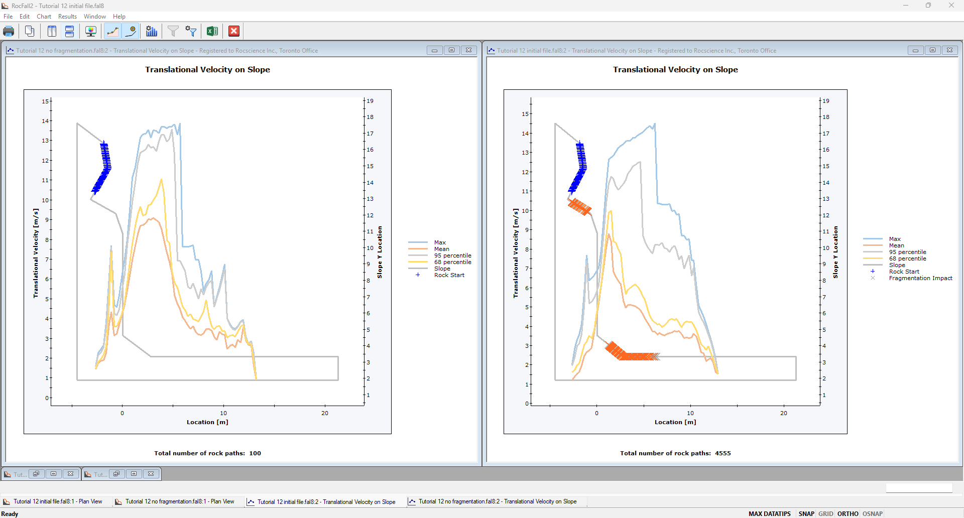
Keep in mind that rotational velocity is not being considered in the two analyses so the total kinetic energy is a function of the rock mass and translational velocity (total kinetic energy equals the translational kinetic energy). For the case with fragmentation, there was a drop in total kinetic energy at the first fragmentation location, mainly due to a reduction in the rock mass of the fragments. Near the slope toe where fragmentation also occurred, the decrease in translational velocity also contributed to a decrease in total kinetic energy.

7. Lastly, let’s compare the runout distances for the two cases. For each model, select Graphs > Graph Endpoints . As the Data to Plot select Endpoint Location, as the Value select Percent of Rocks, and click Plot Data.

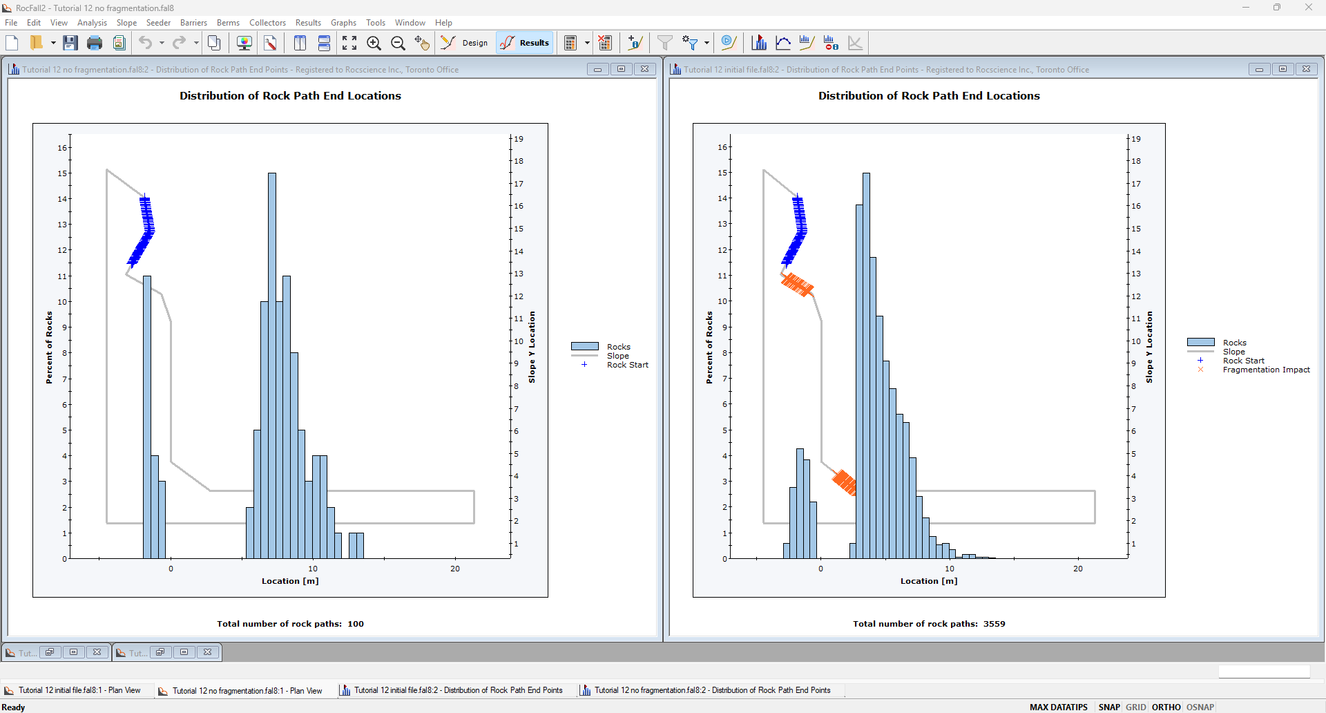
For the case with fragmentation, a greater percentage of rocks ended before x-location = 5 m and a smaller percentage of rocks ended after x-location = 10 m.