2 - Rock Shapes
1.0 Introduction
In this tutorial, the Rigid Body analysis method will be used to define rock shapes in RocFall2, focusing on the effect of rock shape and size.
Topics Covered in this Tutorial:
- Importing DXP files
- Using different shapes
- Defining slope materials
- Filtering paths
Finished Product:
The finished product of this tutorial can be found in the Tutorial 02 Rock Shapes data file. All tutorial files installed with RocFall2 can be accessed by selecting File > Recent Folders > Tutorials Folder from the RocFall2 main menu.
2.0 Model
2.1 IMPORT DXF
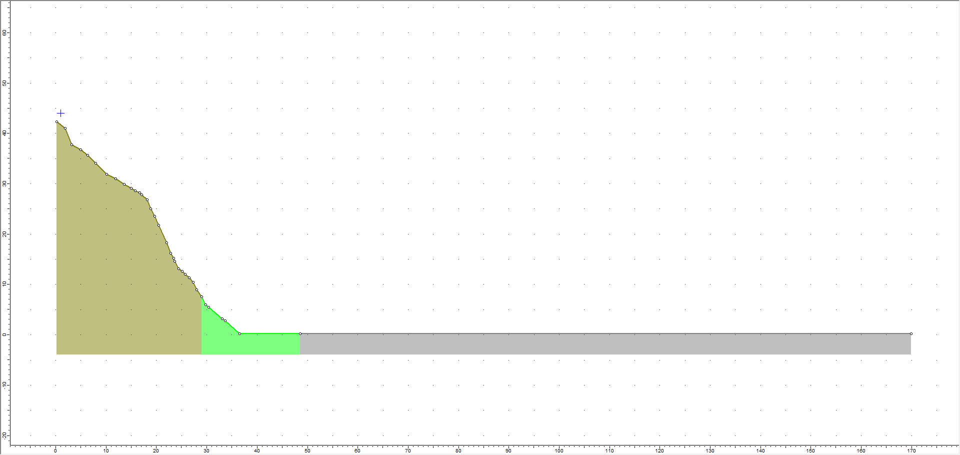
For this example, slope coordinates will be imported from a DXF file using the Import DXF option on the File > Import menu.
- Select: File > Import > Import DXF...
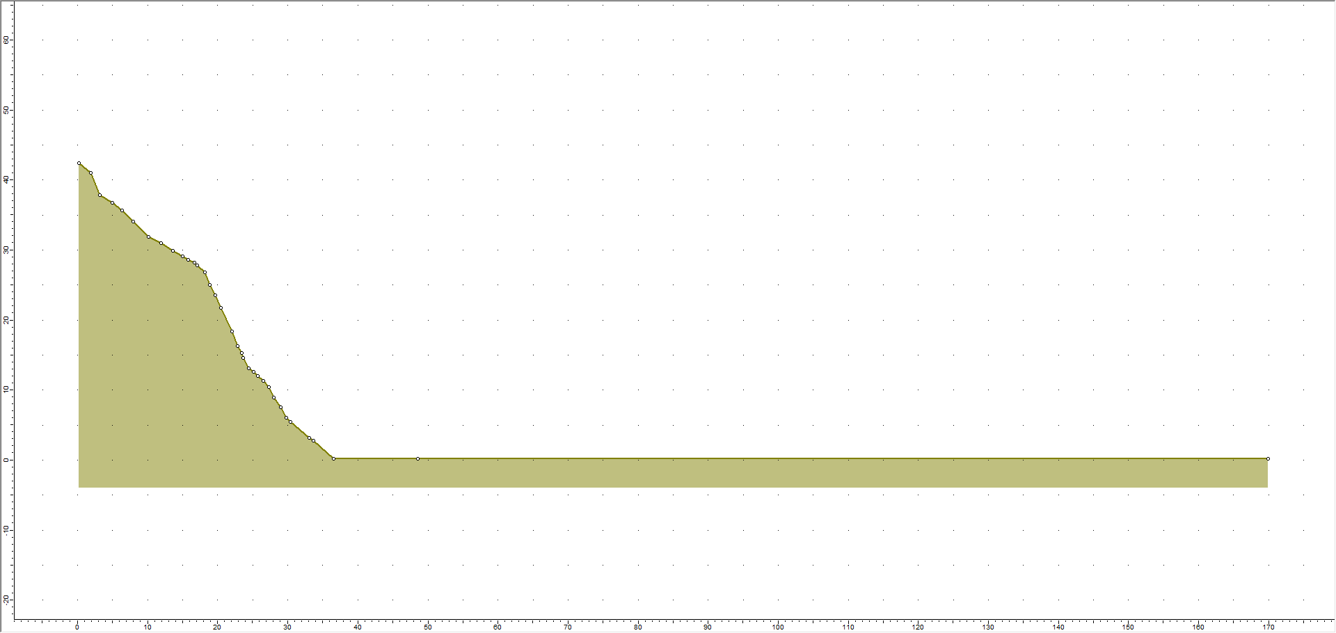
If necessary, navigate to the installation folder: C:\Users\Public\Documents\Rocscience\RocFall Examples\Tutorials, and open the file Tutorial 02_slope_profile.dxf. - Click OK.
The slope should look as follows:
2.2 SPECIFY PROJECT SETTINGS
The Project Settings dialog is used to configure the main analysis parameters of the model. To open the dialog:
- Select: Analysis > Project Settings

The default Analysis Method is Lump Mass. With this method, rocks are assumed to be very small point masses. To use rock shapes, the Rigid Body method must be used.
- Select Rigid Body as the Analysis Method.
- Set Units = Metric (m, kg, kJ).
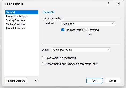
- Click OK.
2.3 DEFINE ROCK TYPES
First, let’s define the rock types for the analysis. Rock Types (Groups) are defined in the Rock Type Library dialog. To open the dialog:
- Select: Seeder > Rock Type Library

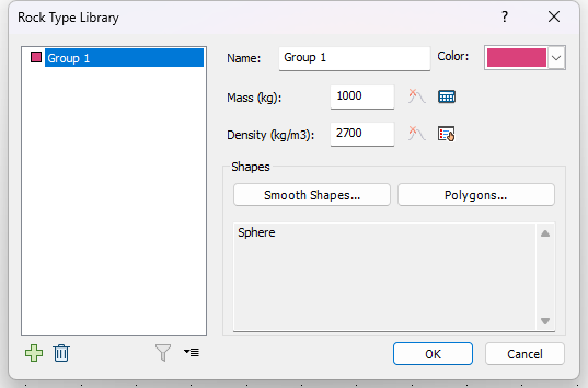
- In the dialog, change the name of Group 1 to Small rocks.
- Click the Smooth Shapes button.
The Smooth Shapes popup appears.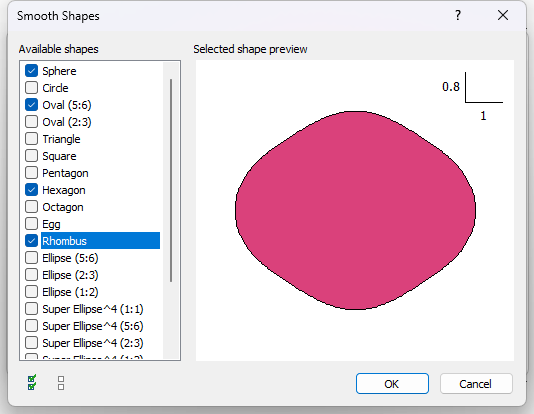
- In the Available Shapes list, select Sphere, Oval (5:6), Hexagon, and Rhombus.
- Click OK.
Back in the Rock Type Library dialog, let's define the Distribution for Mass, Density, and Initial Rotation of the rocks for the Small rocks group:
- Ensure Mass (kg) = 1000.
- Click the Distribution icon
 next to Mass and set the parameters as shown below:
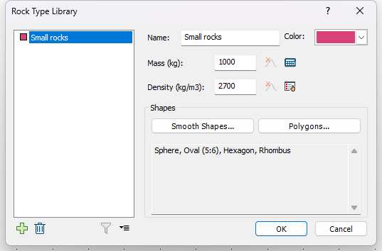
By default, 3x std. dev. is selected to calculate the relative minimum and maximum to be three times the standard deviation; these values can be changed manually if necessary. - Set Density (kg/m3) = 2700.
- Click the Distribution icon next to Density .
- Set Distribution = Normal and Std. Dev: = 50, and leave 3x std. dev. selected.
- Click OK.
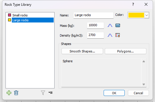
Back in the Rock Type Library dialog, let’s add a second rock type:
- Click the Add button in the bottom-left corner of the dialog.
- Rename the new type as Large rocks.
- Set Mass (kg) = 10000.
- Click the Distribution icon next to Mass and set the parameters as shown below:
- Click OK.
- Set Density (kg/m3) = 2700.
- Click the Distribution icon next to Density .
- Set Distribution = Normal and Std. Dev: = 50, and leave 3x std. dev. selected.
- Click OK.
- Click the Smooth Shapes button to open the Smooth Shapes dialog.
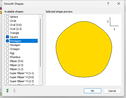
- In the Available Shapes list, select Square and Pentagon.
- Click OK in the Smooth Shapes dialog.
- Click OK in the Rock Type Library dialog.
2.4 DEFINE SEEDER
Next we'll define a Point Seeder to specify the initial conditions of the falling rocks, using the Add Point Seeder option and the Seeder Properties dialog.
- Select: Seeder > Add Point Seeder

- In the prompt line at the bottom-right of the application window, enter the coordinates (1, 44).
The Seeder Properties dialog appears. - Keep Seeder Name as Seeder 1 and set Number of Rocks = 100.
- Ensure both Small rocks and Large rocks are selected in the Rock Types list.
- Set Horizontal Velocity (m/s) = 3.
- Click the Distribution icon next to Horizontal Velocity and set Distribution = Normal and Std. Dev: = 0.4. Leave 3x std. dev. selected.
- Leave Vertical Velocity (m/s) and Rotational Velocity (m/s) as 0 with Distribution = None.
- Set Initial Rotation = 0 and set Distribution = Uniform.
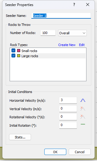
- Click OK.
2.5 DEFINE SLOPE MATERIALS
Next we'll define slope materials using the Slope Material Library. For this tutorial, we'll keep the three default materials. To view the materials:
- Select: Slope > Slope Material Library

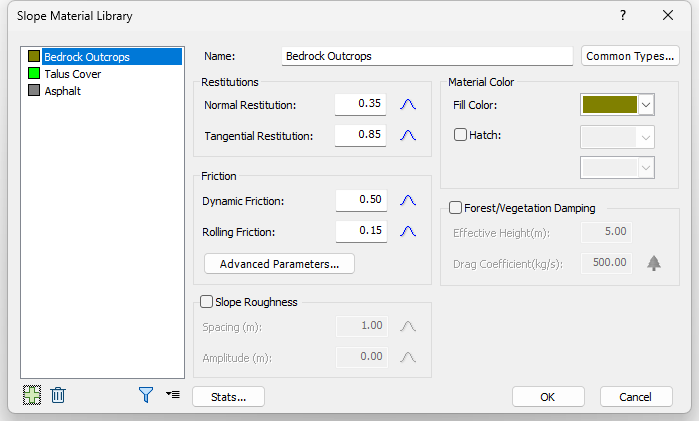
- Click Cancel to close the dialog.
2.6 ASSIGN SLOPE MATERIALS
Now we'll assign slope materials to the model according to the figure below:
To assign materials:
- Select Assign Materials
 on the Slope menu or the toolbar.
The Assign Materials dialog appears.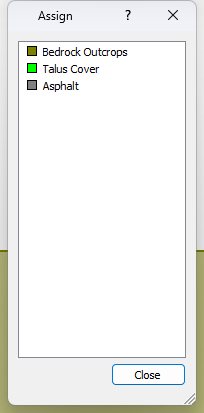
- In the dialog, click the material you want to assign.
- On the model, click the slope line segments to which you want to assign the material.
- Repeat the steps above until you have finished assigning materials to the model as shown.
- Close the Assign Materials dialog.
3.0 Results
Finally, we'll run the analysis. To do that, you must you must first run Compute. To Compute:
- Select the Compute
 option from the toolbar or the Analysis menu.
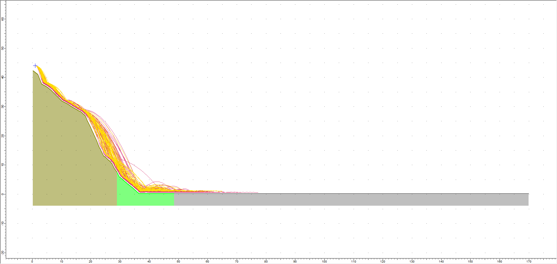
You should see the figure below showing the rock paths on the slope. The Analysis Tools should also now be available on the toolbar and the main menu.
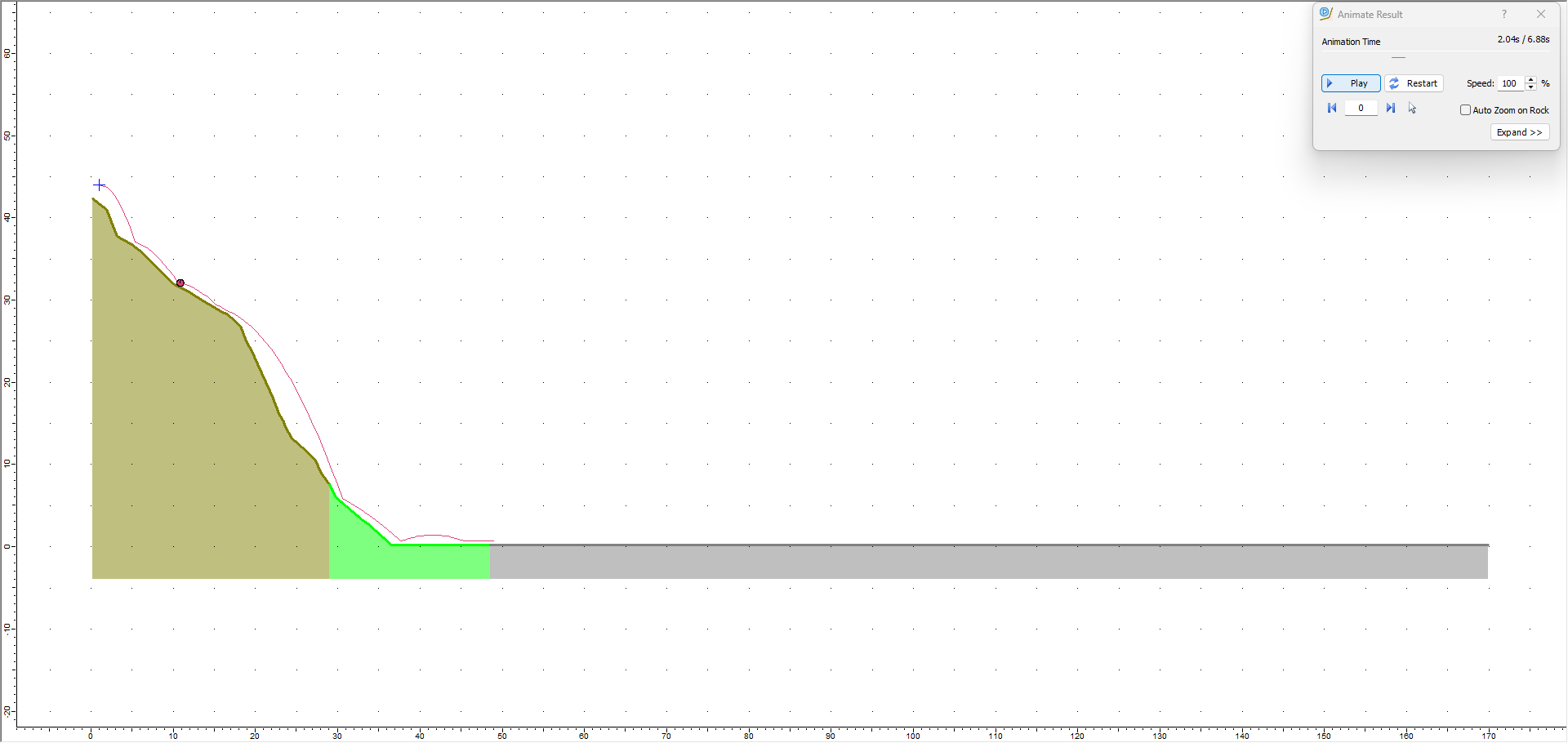
3.1 ANIMATE PATHS
A very useful feature of RocFall2 is the ability to animate the path individual rocks on your model take as they fall using the Animate Result dialog.
To animate rock paths:
- Right click on any rock path and select Animate Path
 .
.
Observe how the rock shape travels down the slope. The gold paths represent the Large Rocks Rock Type.
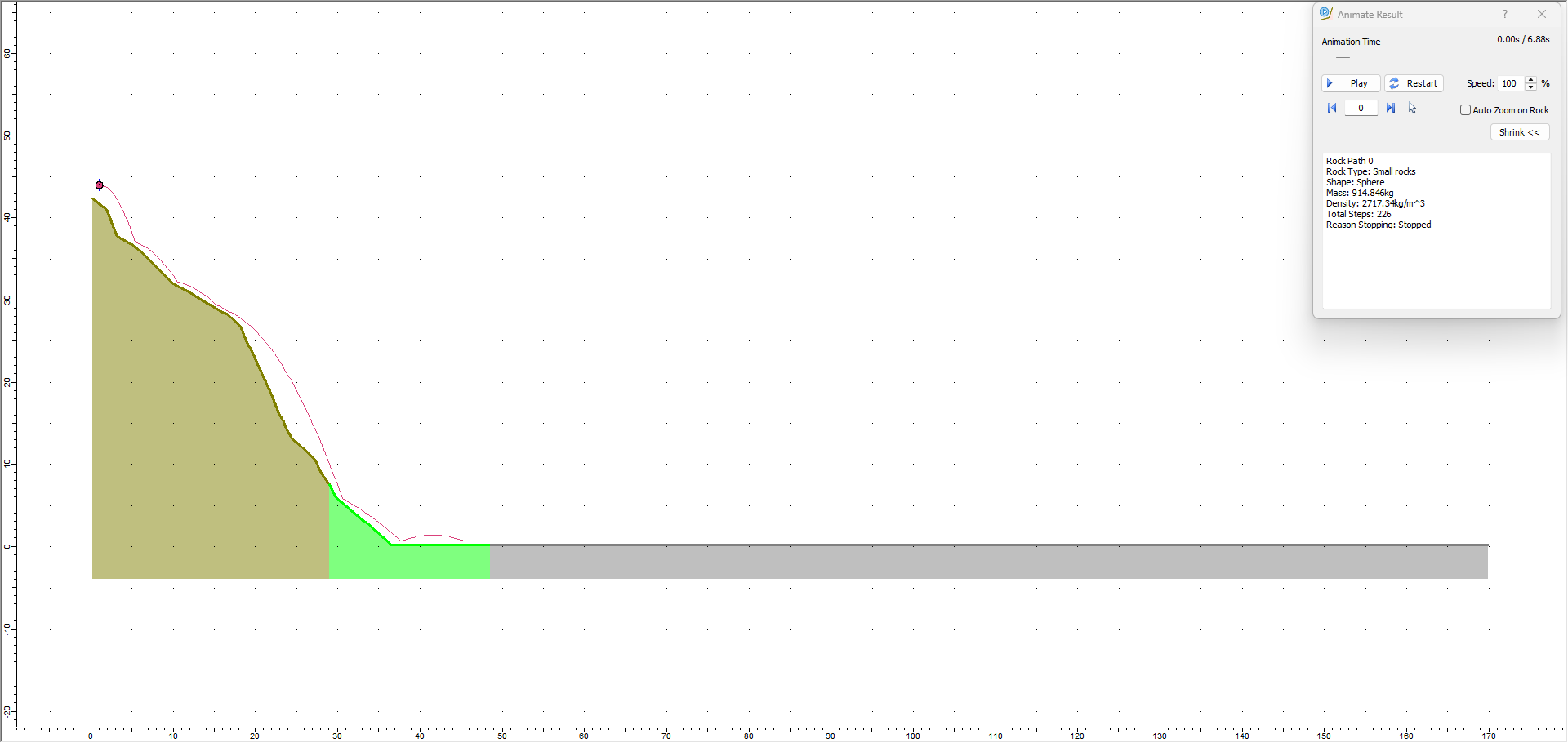
To cycle through each rock in the model and animate its path:
- In the Animate Result dialog, click through different rock paths using the forward arrow beside the rock ID number.
The rock ID numbers can be used to differentiate the Large Rocks (50-99)from the Small Rocks (0-49). - Click the Expand button in the dialog to display information about the current rock (i.e., rock shape and mass) as shown in the figure below.
To view the contact points of a rock shape:
- Right-click on the rock's path and select Display Contacts. Zoom in to the contact points to see them more clearly
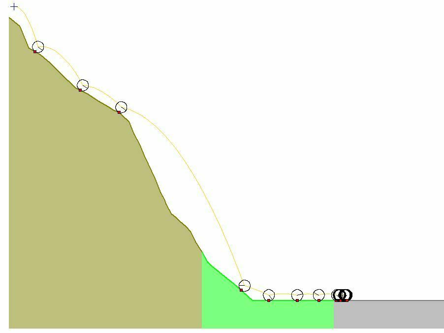
3.1.1 Rigid Body vs. Lump Mass Rock Paths
A frequently asked question for the Rigid Body analysis is, “why are the rock paths hovering above the slope??”
With the Rigid Body analysis method, it is important to note that the rock paths represent the path of the centroid of each rock shape. Therefore, the rock paths do not touch the slope, even when the rock shapes are in sliding or rolling mode along slope segments.
With the Lump Mass analysis method, since the rocks do not have a physical size, the paths overlap the slope segments when the rocks are in sliding or rolling mode.
3.2 GRAPH ENDPOINTS
Now we'll create a graph of the rock endpoint locations by selecting Graph Endpoints ![]() from the Graphs menu or from the toolbar. The horizontal axis of the Distribution of Rock Path End Locations graph is the x-coordinate of the slope and the vertical axis is the number of rocks that ended in the bin at that location.
from the Graphs menu or from the toolbar. The horizontal axis of the Distribution of Rock Path End Locations graph is the x-coordinate of the slope and the vertical axis is the number of rocks that ended in the bin at that location.
To create the graph:
- Select: Graphs > Graph Endpoints
 .The Graph Endpoints dialog should appear.
 - Set Data = Endpoint Location.
- Set Value = Number of Rocks.
- Set Number of Bins = 50.
- Set Paths to Plot = All Rock Paths.
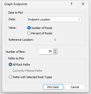
- Select Plot Data to generate the Distribution of Rock Path End Locations graph.
- Select Tile Horizontally on the toolbar or the Window menu.
- Click in the slope model and press F2 to Zoom All.
You should see the following.
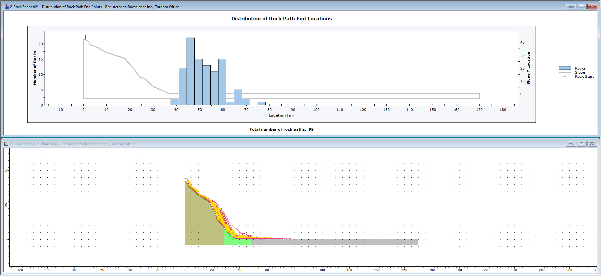
By default, the Endpoints Graph plots the end locations of all rocks regardless of the rock type.
3.3 FILTER RESULTS
You can use the Filter Results dialog to filter results by rock type, rock shape, and other criteria. To open the dialog:
- Select: Results > Filter Options

- Under Available Filters, select Rock Type.
- In the Rock Type drop-down, select Small rocks and click OK.
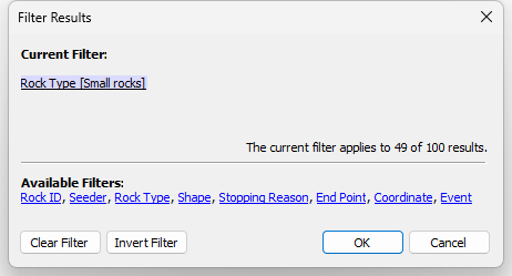
Filter Results Dialog 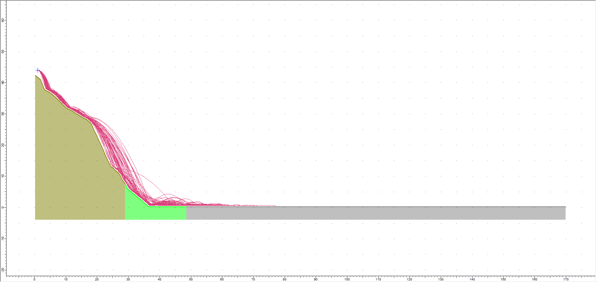
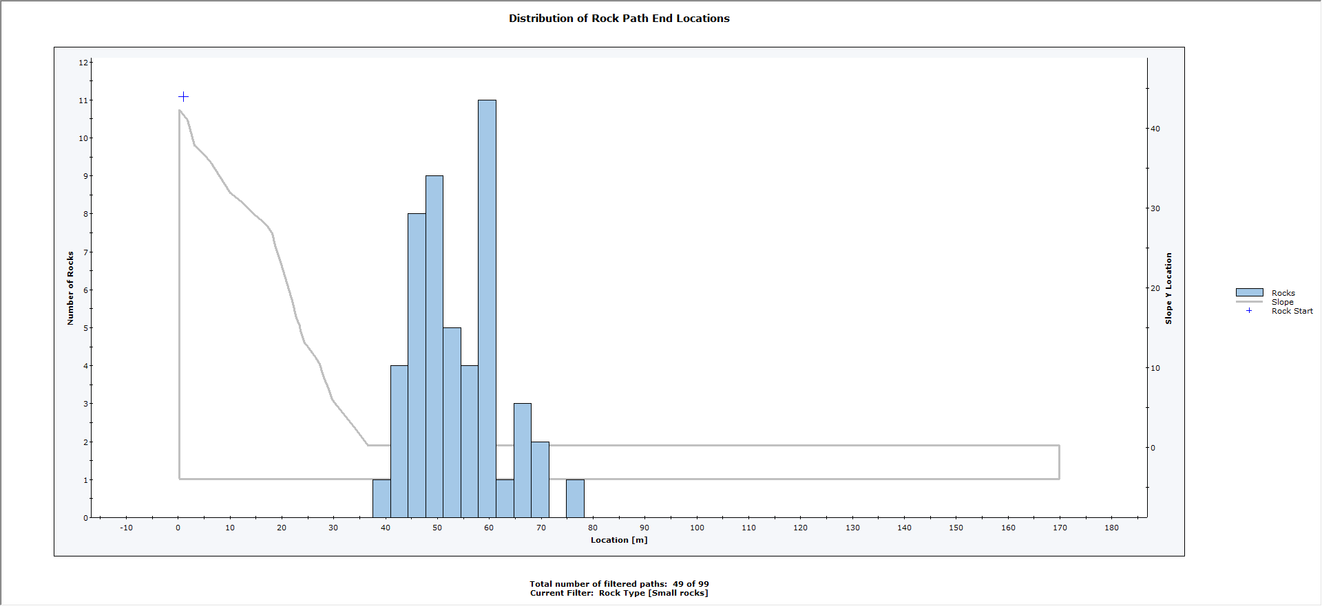
Results Filter View - Click OK and view the Endpoints histogram with the filter applied.
- Re-open the Filter Results dialog.
- Select Large rocks as the Rock Type as above.
Now let's filter on Large rocks:
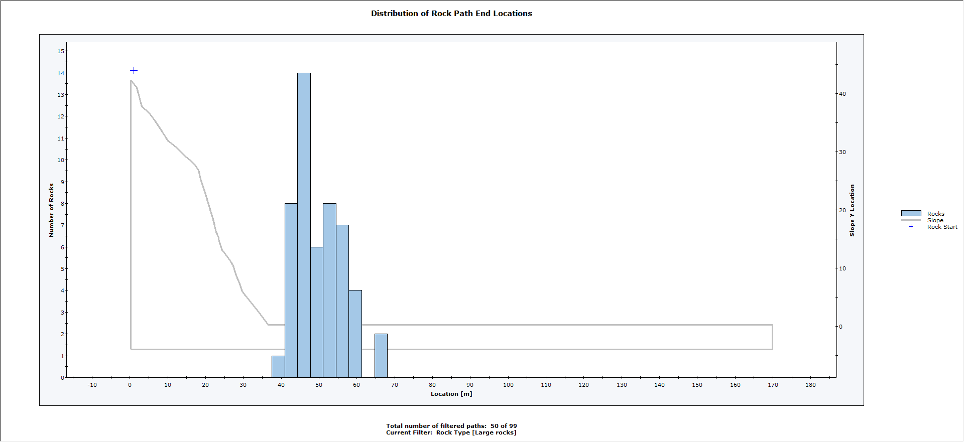
The filtered results show that the small rocks have a broader distribution of endpoints and, on average, travel farther than the large rocks. However, since different rock shapes were used for the large and small rocks, this must be considered as well.
3.4 ENVELOPE GRAPHS
Now let's generate a Total Kinetic Energy graph using the Graph Data on Slope dialog.
- Select: Graphs > Graph Data on Slope

- In the dialog, set Data = Total Kinetic Energy.
- Set Paths to Plot = Paths with Selected Rocks.
- Leave both Small rocks and Large rocks selected.
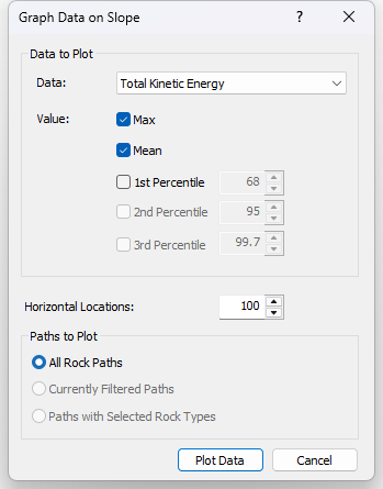
- Click Plot Data.
You should see the following graph.
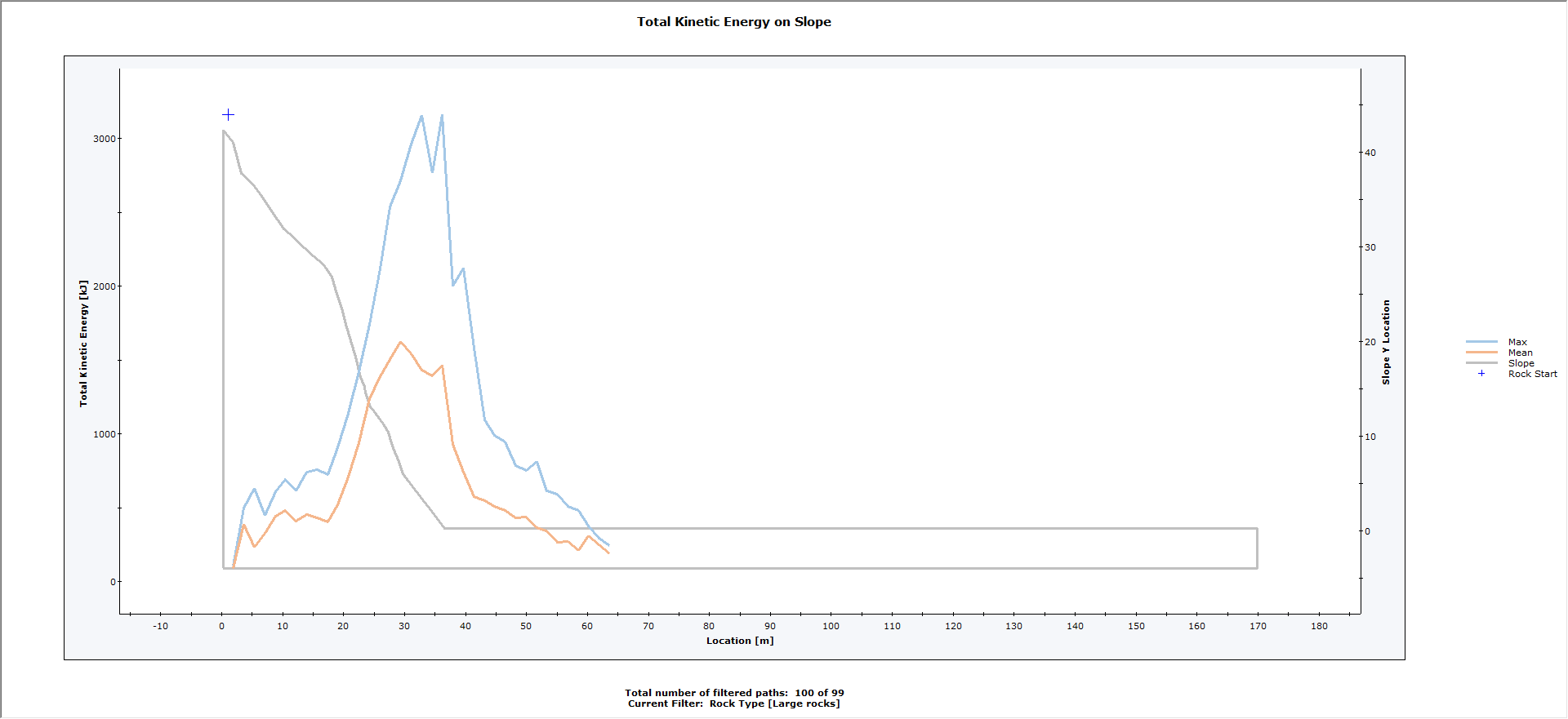
NOTES:
- Notice that Rock Types are separated into different series when they are plotted in the graph. To plot one series at a time, return to the Graph Data on Slope dialog to select only one rock type.
- Since we are plotting Kinetic Energy, you can see that the energy of the Large rocks (red curve) is much greater than the Small rocks (blue curve) since the Large rocks are 10 times heavier on average.
This concludes the tutorial. You are now ready for the next tutorial, Tutorial 03 - Barriers and Collectors in RocFall2.