1 - Quick Start

1.0 Introduction

This tutorial is a simple introductory tutorial that helps you become familiar with the basic modeling and data interpretation features of RocFall2. RocFall2 is a 2D statistical analysis program designed to assist with assessment of slopes at risk for rockfalls.

Topics Covered in this Tutorial:

• Creating/editing slopes
• Defining/editing seeders
• Assigning slope materials
• Animation tool
• Analysis tools

Finished Product:

The finished product of this tutorial can be found in the Tutorial 01 Quick Start data file. All tutorial files installed with RocFall2 can be accessed by selecting File > Recent Folders > Tutorials Folder from the RocFall2 main menu.

2.0 Creating a RocFall2 File

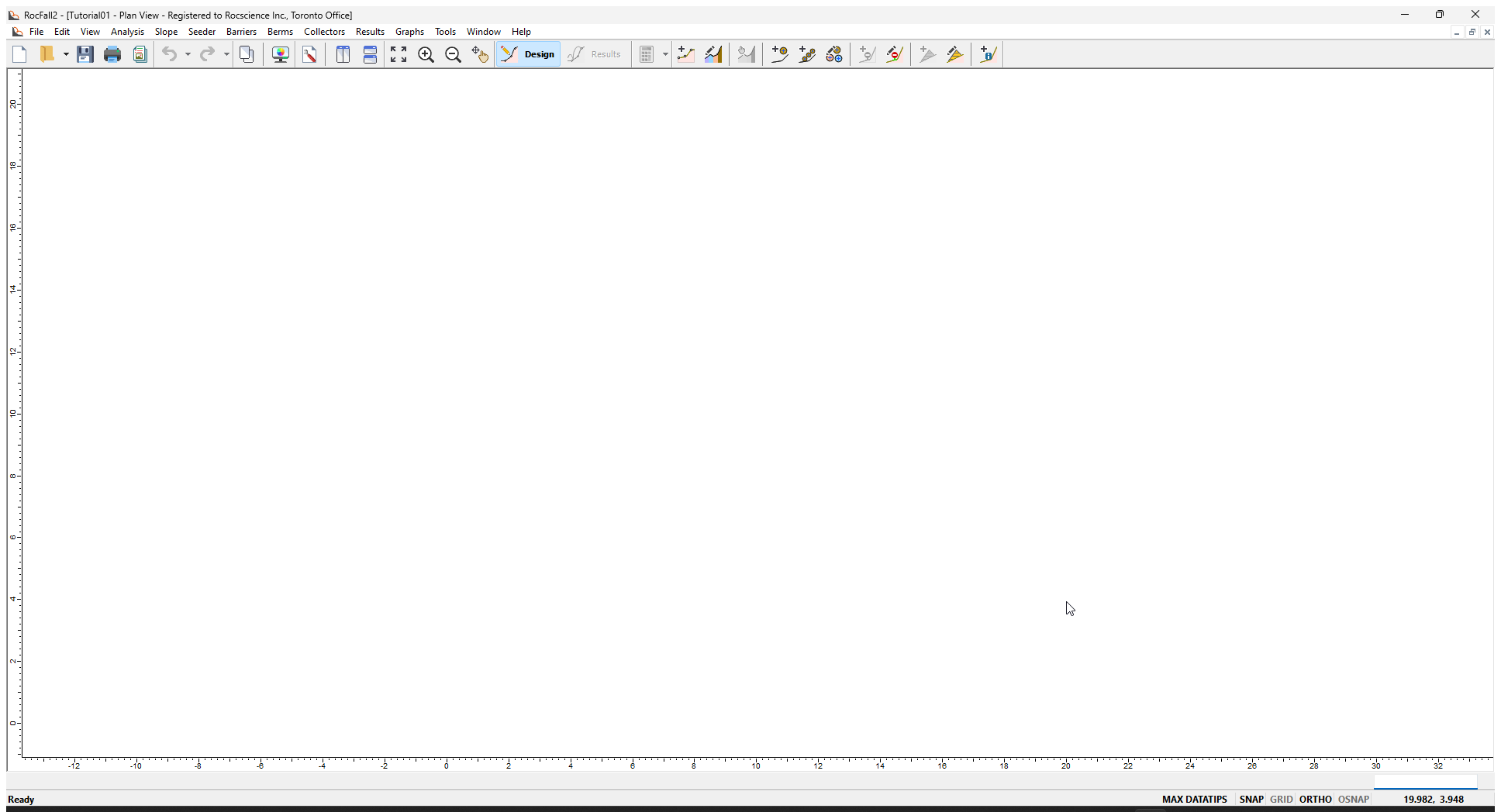
1. Start RocFall2 by selecting Programs > Rocscience RocFall2 > RocFall2 from the Windows Start menu.

RocFall2 automatically opens a new blank document, which allows you to begin creating a model immediately. If the RocFall2 application window is not already maximized, maximize it now so the full screen space is available for use.

3.0 Model

3.1 PROJECT SETTINGS

The Project Settings dialog is used to configure the main analysis parameters of the model. To open the dialog:

1. Select: Analysis > Project Settings

3.1.1 Analysis Method

In RocFall2 there are two possible Analysis Methods to choose from in the General tab: Lumped Mass and Rigid Body.

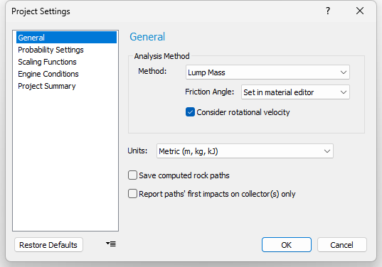
• The default method is Lump Mass. With the Lump Mass method, the rocks are assumed to be very small point masses with no physical size.
• The Rigid Body analysis method allows you to define rock shapes. Rock shapes are covered in later tutorials.

1. We will be using the Lump Mass method for this tutorial.

3.1.2 Engine Conditions

1. Select the Engine Conditions tab.

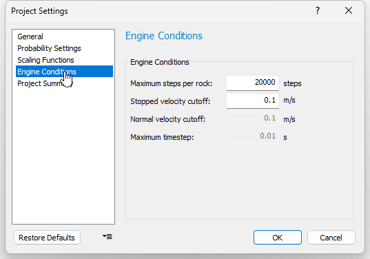
Note the various control parameters. Once one of these conditions is met, the rock will stop moving. For more help on engine stopping conditions, see Engine Stopping Conditions Settings in RocFall2.

2. For this tutorial, leave the default settings.
3. Click OK.

3.2 CREATING / EDITING THE SLOPE

In RocFall2, the slope can be drawn either manually with the cursor using Add Slope or by inputting vertex coordinates using the Edit Boundary Coordinates dialog. Both options are on the Slope menu. In this tutorial, we are going to input coordinates to draw the slope.

NOTE: You must be in Design mode to draw or edit the slope geometry. To enable Design mode, select the Design icon on the toolbar.

To open the Edit Boundary Coordinates dialog:

1. Select: Slope > Edit Coordinates



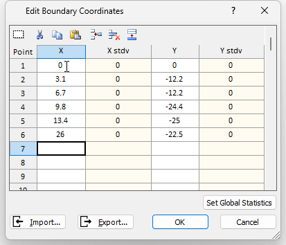
2. Enter the coordinates as shown above.
3. Click OK.

Press F2 to Zoom All. The slope geometry should appear as shown below.

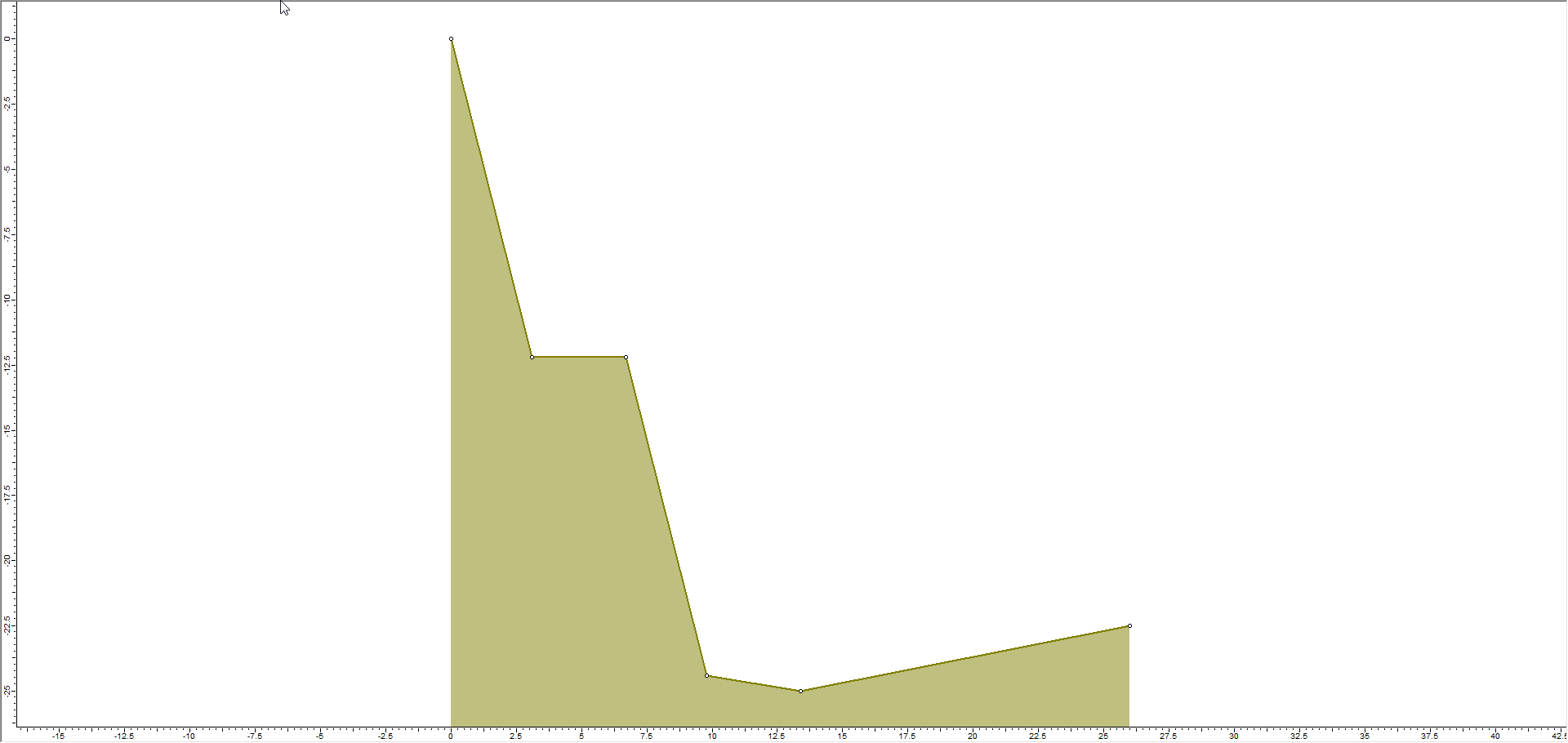
You can always open the Edit Boundary Coordinates dialog by right clicking on the slope and selecting Edit Slope Coordinates. You can also manually move vertices or delete them using right-click shortcuts.

3.3 ADDING / EDITING SEEDERS

In RocFall2, seeders determine the drop location for rocks. You add seeders to your model using the Add Point Seeder option on the toolbar or Seeder menu.

1. Select: Seeder > Add Point Seeder

You can place a seeder at a location using the cursor on the screen or by entering the coordinates in the prompt line. The prompt line is located at the bottom right of the RocFall2 application window and it is commonly used for entering coordinates while creating the slope geometry.

2. Enter 0.5, 0 in the prompt line.
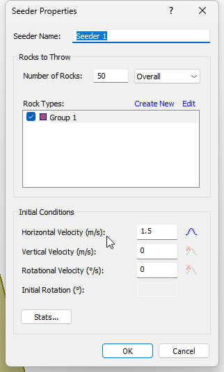
   The Seeder Properties dialog should appear.
3. In the dialog, select Group 1 from the rock type list on the left-hand side.
4. Change Number of Rocks to 50.

You can also use this dialog to define the initial Velocity of each rock group. You can set the mean, standard deviation, and relative minimum and maximum for the initial velocity to get the desired distribution.

5. Set the mean value for Horizontal Velocity to 1.5.
6. Click the Distribution icon next to the value.
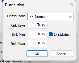
7. Change Distribution to Normal.
8. Set Std. Dev: to 0.15.
9. Select the 3x std. dev. check box to automatically calculate the Rel. Min: and Rel. Max values to three times the entered standard deviation OR enter the values manually.
   
10. Set Vertical Velocity = 0 and Rotational Velocity = 0, and leave Distribution for both set to None.
    For the Lump Mass method, the Initial Rotation is not applicable, so it is disabled (initial rotation is only applicable for rigid body rock shapes).
11. Click OK.

3.4 ROCK TYPES

Let's now look at the rock properties of the model. Rock properties are set up through the Rock Type Library dialog. To open the dialog:

1. Select: Seeder > Rock Type Library

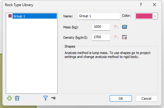
In this dialog, we can create different rock types (Groups) and define the Mass and Density of each one. You can also use the dialog to define rock Shapes if the Analysis Method = Rigid Body. Since we are using the Lump Mass method, rock shapes are not available.

2. Leave the default settings for Group 1.
3. Click OK.

3.5 DEFINING SLOPE MATERIALS

Next, let's define slope materials using the Slope Material Library dialog. To open the dialog:

1. Select: Slope > Slope Material Library

Similar to the Seeder Properties dialog, the Slope Material Library dialog allows you to change the distribution type and the distribution parameters for each material. You can also add or remove materials.

Let's define three new materials:

2. Click the Add button in the Slope Material Library dialog to create a new material type.
3. Change the name of the new material to Type One and enter the properties given in the table below.
4. Repeat steps 1 and 2 to define two more new materials named Type Two and Type Three. See the table below for their properties:

Name	Normal Restitution (mean | sd)	Tangential Restitution (mean | sd)	Friction (mean | sd)
Distribution	Normal	Normal	None
Type One	0.5 | 0.03	0.9 | 0.03	30 | 0
Type Two	0.4 | 0.03	0.9 | 0.03	30 | 0
Type Three	0.3 | 0.03	0.9 | 0.03	30 | 0

5. When you are finished entering all of the properties, the dialog should look as follows:



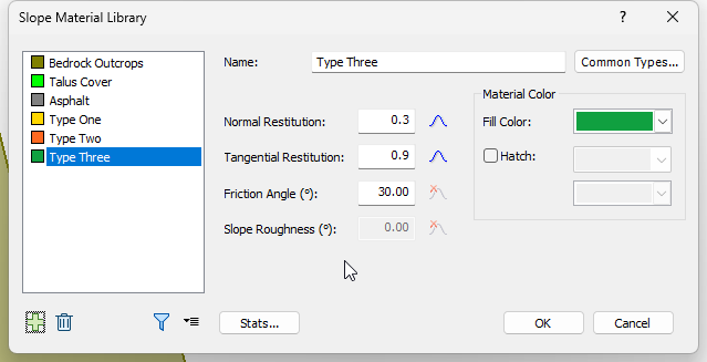
6. Click OK.

3.6 ASSIGNING SLOPE MATERIALS

You are now ready to assign the material properties to the slope using the Assign Slope Materials dialog. To open the dialog:

1. Select: Slope > Assign Slope Materials



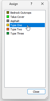
2. Select Type One on the list.
3. Left-click on the first and third line segments from the left on the model to assign them the Type One material.
4. Select Type Two and left-click on the second segment from the left.
5. Select Type Three and left-click on the last two segments.
6. Close the dialog.

The model should appear as follows: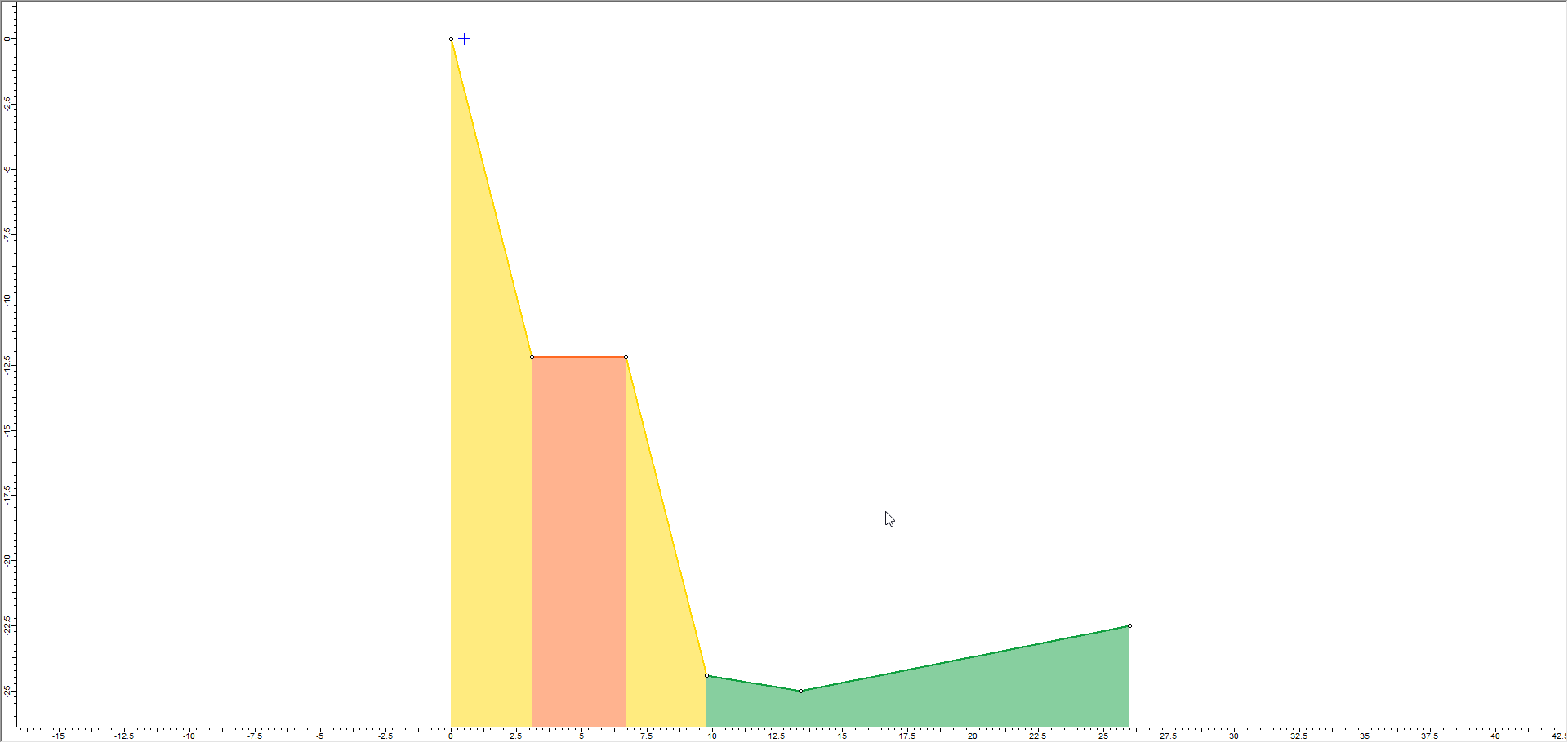

4.0 Results

To view analysis results in RocFall2 you must first run Compute.

1. To Compute, select the Compute option from the toolbar or the Analysis menu.
2. After compute is complete, the view will be switched to Results mode automatically. In this mode, the analysis tools appear on the main toolbar and the rock paths are shown on the slope.

The image below shows the results of 50 rock throws using the Lump Mass analysis method.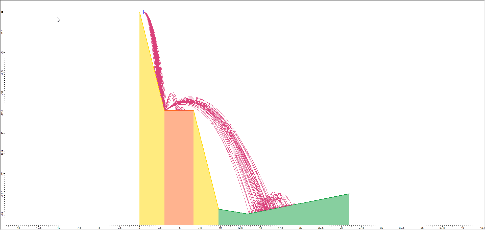

4.1 ANIMATING ROCK PATHS

A very useful feature of RocFall2 is the ability to animate the path individual rocks on your model take as they fall using the Animate Result dialog. To open the dialog and animate the rock paths:

1. Select: Results > Animate Path.

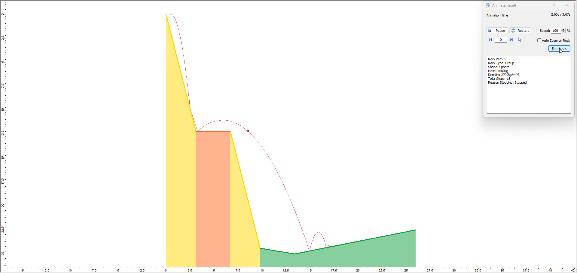
2. In the dialog, click the Back and Forward arrows to cycle through each rock in the model (Rock ID) and play its animation.
   The rock path variability for this example, is generated by the statistical distributions we defined for the initial velocity of the rocks, and the slope material properties.
3. Use the Speed setting to change the speed of the animation.
4. Select the Auto Zoom on Rock check box to zoom in on the selected rock while watching the animation.
5. Click Expand to view details of the selected rock and its animation.
6. Close the dialog.

4.2 VISUALIZING RESULTS WITH GRAPHING TOOLS

RocFall2 has a number of graphing tools that allow you to visualize the results of the analysis. The tools are available on the toolbar and the Graphs menu. For this tutorial, we'll look at the following tools: Graph Endpoints, Graph Data on Slope, and Graph Distribution.

4.2.1 Graphing Endpoint Locations

Graphing the horizontal location of rock endpoints is one of the most common and easily understood results from a RocFall2 analysis.

To graph Location Endpoints:

1. Select: Graphs > Graph Endpoints

The Graph Endpoints dialog should appear.

2. Set Data = Endpoint Location.
3. Set Value = Number of Rocks.
4. Set Number of Bins = 50.
5. Set Paths to Plot = All Rock Paths.



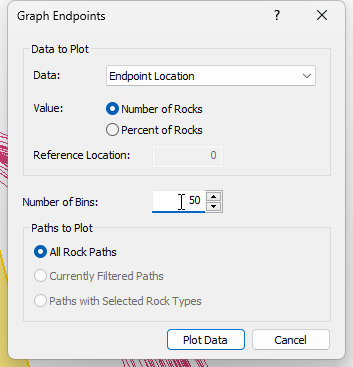
6. Select Plot Data to generate the Distribution of Rock Path End Locations graph.
7. Select Tile Windows on the toolbar (Tile Horizontally on the Window menu) to view the model (the Plan View) and the Distribution of Rock Path End Locations graph side-by-side.
8. Right-click on the model to open the right-click menu.
9. Select Zoom All (you can also press F2).

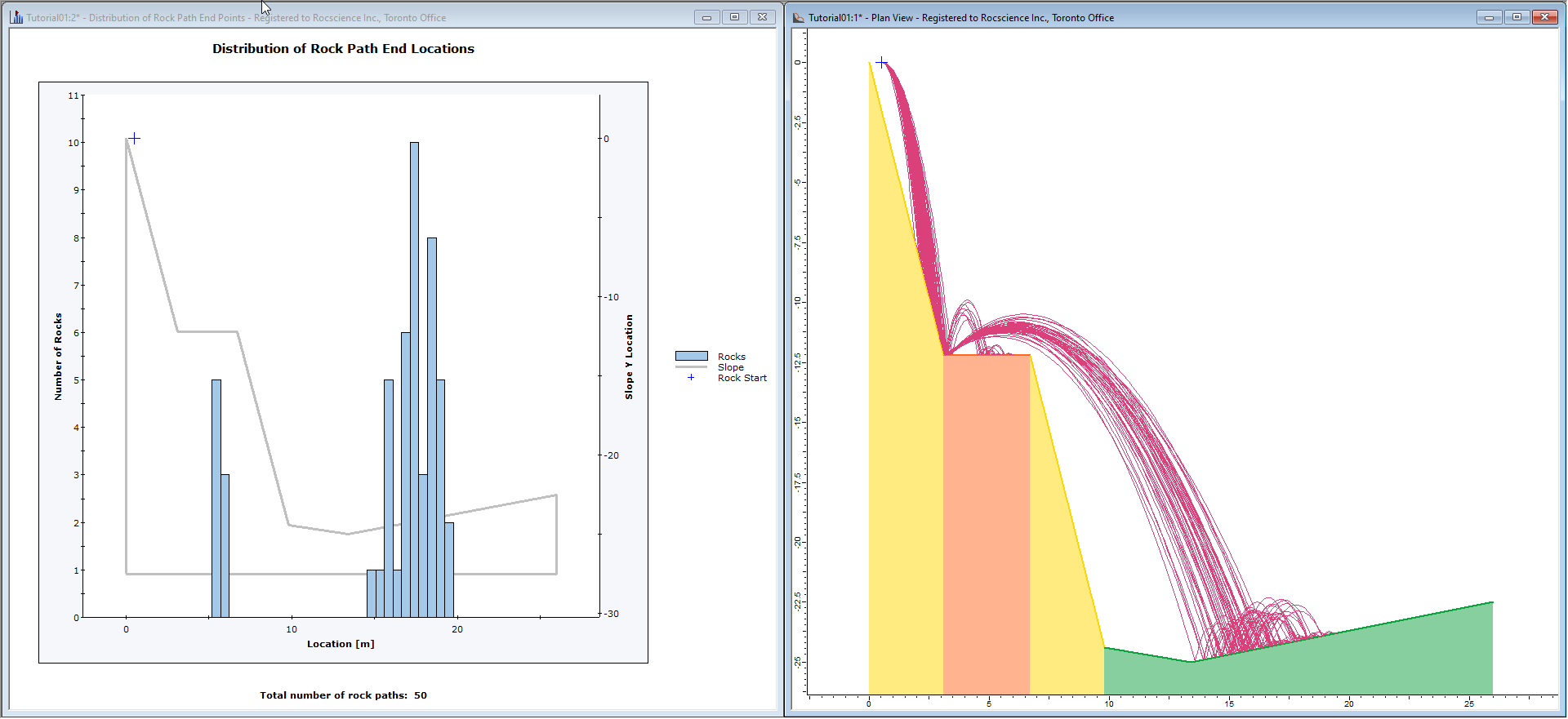
As you can see from the endpoint histogram, most rocks come to rest at the bottom of the slope, but a few have stopped on the upper bench.

4.2.2 Graphing Data on the Slope

Envelope graphs of rockfall results can be generated with the Graph Data on Slope option. Kinetic Energy (Total, Translational, and Rotational), Velocity (Translational and Rotational) and Bounce Height envelopes can be generated.

To graph Bounce Height on the slope:

1. Select: Graphs > Graph Data on Slope

The Graph Data on Slope dialog should appear.



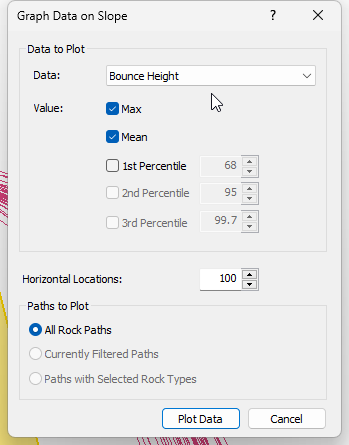
2. Select Bounce Height as the Data to Plot.
3. Change the Data to Plot Value to Max.
4. Select Plot Data.

Note that the plot will appear in a new tab and you can switch back to the slope view tab to carry out other analyses.

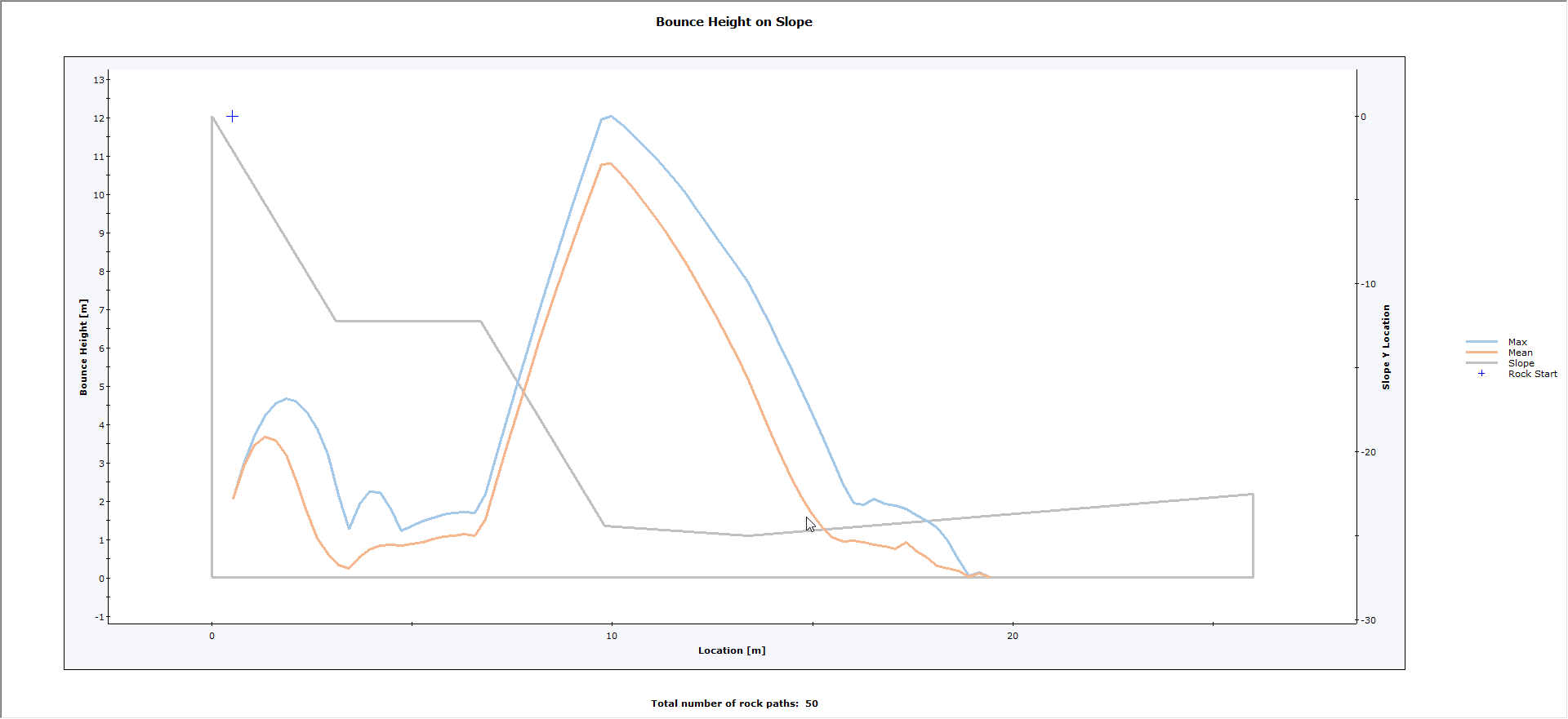
Note that you can also specify the Mean or a Percentile value to plot, since the Max is generally conservative.

4.2.3 Graphing Distributions

Distribution graphs show the distribution of results at a selected X-location (horizontal location) along the slope. Kinetic Energy (Total, Translational, and Rotational), Velocity (Translational and Rotational) and Bounce Height distribution graphs can be generated.

To graph the Translational Kinetic Energy distribution:

1. Select: Graphs > Graph Distribution



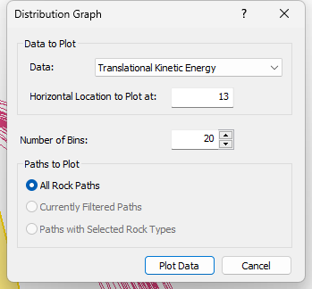
2. In the Distribution Graph dialog, select Translational Kinematic Energy as the Data to Plot.
3. Leave the other settings as is.
4. Select Plot Data.

The results appear in a new tab as a split view as shown.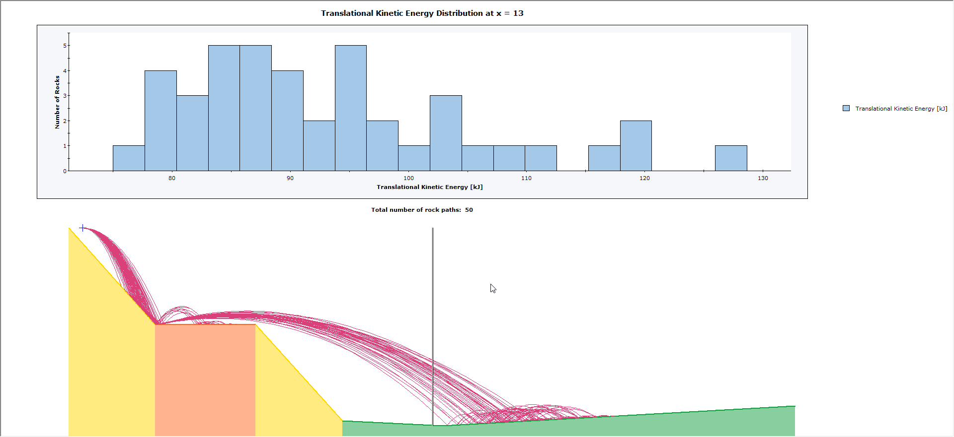

As you click on different locations on the slope model at the bottom of the split view, the chart above will update with the distribution results corresponding to the indicator location. You can click the mouse or click and drag the vertical location indicator to update the graph results.

4.2.4 Exporting Graph Results to Excel and the Clipboard

You can view the data from any graph you generate in Microsoft Excel by selecting Export to Excel on the File menu or by right-clicking on the plot area and selecting Plot in Excel

You can also right-click any plot area and select Copy Data to copy the raw data used to generate graphs to the Windows Clipboard. From the Clipboard, the raw data can be pasted into word processing or spreadsheet programs, for further analysis, or report writing.

This allows you, for example, to perform custom analyses that are not available with RocFall2. For instance, you could copy the raw data associated with the rock endpoints into your spreadsheet, sort the data and fit an unusual probability distribution to the data.

4.3 REPORT GENERATOR LISTING OF MODEL PARAMETERS

The Report Generator displays a summary of all RocFall2 model parameters and summarized results in its own independent app. This includes:

• Slope geometry
• Slope materials
• Seeder properties and rock types
• Simulation parameters
• Barrier and collector properties
• Summary results*
• Generated path details and rock geometries*
• Summary path results*
• Barrier and collector impact results*
• Barrier design reports*
• Added views*

To open the Report Generator:

1. Select: Analysis > Report Generator

The Report Generator information can be copied to the clipboard using the options in the right-click menu. From the Clipboard, the information can be pasted into word processing programs for report writing.

4.4 SAVING THE MODEL

1. Select: File > Save
2. Enter the name QuickTutorial for our file.

This concludes the tutorial. You are now ready for the next, tutorial, Tutorial 02 - Rock Shapes in RocFall2.