This tutorial shows you how to directly apply standard deviations to the coordinates of slope vertices in RocFall2 using the Edit Boundary Coordinates dialog . This allows the model to account for uncertainty in measurements or to simulate a pseudo 3-D rockfall analysis (i.e., to simulate minor variations in a slope profile).
Topics Covered in this Tutorial:
Constant seeder/slope properties
Editing slope coordinates
X, Y vertex variation
Finished Product:
The finished product of this tutorial can be found in the Tutorial 04 Vertex Variation data file. All tutorial files installed with RocFall2 can be accessed by selecting File > Recent Folders > Tutorials Folder from the RocFall2 main menu.
2.0 Model
2.1 OPEN THE TUTORIAL FILE
Let's start by opening the file for the tutorial:
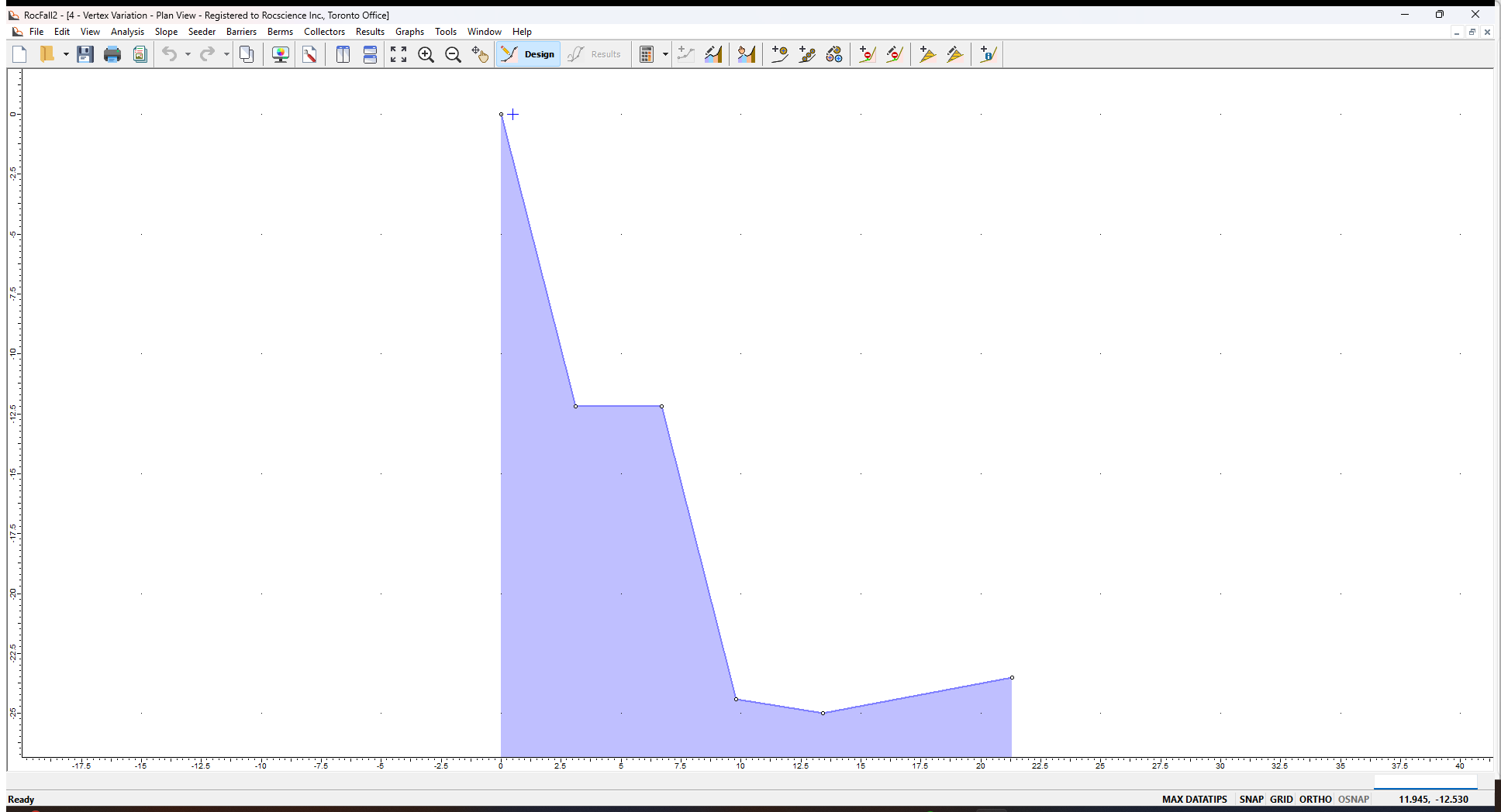
Select: File > Recent Folders > Tutorials Folder and open the Tutorial 04 initial file. You should see the following model.
All slope and rock properties have already been defined, except for the vertex variation:
The Rigid Body rock shape is a 1000 kg sphere
Number of rocks = 50
The vertex variation has not been defined
Let’s first review the properties of this model.
2.2 SEEDER PROPERTIES
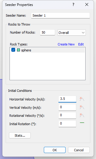
You can view the properties of the existing point seeder in the Seeder Properties dialog:
Right-click the point seeder on the model (the blue cross at the top of the slope) and select Seeder Properties in the popup menu.
Note the following:
Number of Rocks = 50
Initial Horizontal Velocity (m/s) = 3.5
No statistical distribution has been defined for the initial velocity, so all rocks will follow the same initial path
Click Cancel to close the dialog.
2.3 SLOPE MATERIAL PROPERTIES
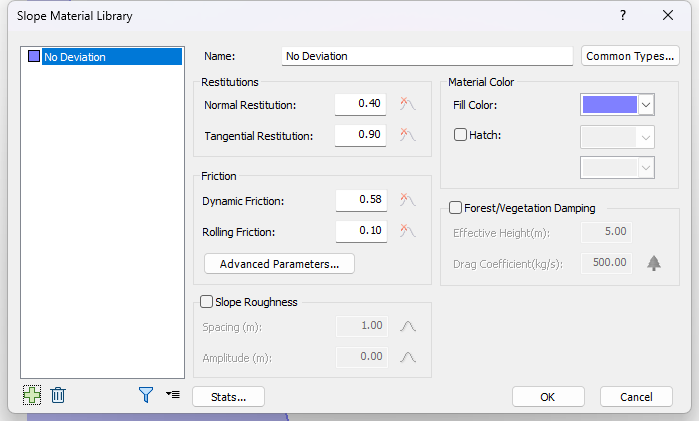
Next we'll look at the slope materials properties in the Slope Material Library dialog.
Select Slope Material Libraryon the toolbar or the Slope menu.
Note the following:
A single material named No Deviation has been defined.
The Distribution of all parameters is set to None.
Click Cancel to close the dialog.
3.0 Results
Now we'll run Compute and then use the Animate Path option to view the rock fall.
Select Compute from the toolbar or the Analysis menu.
Select Animate Path on the toolbar or the Results menu.
In the Animate Result dialog, click Play. You should see only a single rock path travel down the slope.
Since there is no statistical variation (Distribution = None) in the rock's Initial Conditions, all 50 rocks have the same path so only that path is shown and animated.
4.0 Model Vertex Variation
Now we will demonstrate how to apply geometric variability to the slope coordinates by applying standard deviations to the slope vertices.
Select Design on the toolbar.
Select Edit Coordinates on the Slope menu or right-click on the slope and select Edit Slope Coordinates.
For Point (Vertex) 3 (mean coordinates = 6.7, –12.2), enter X stdv = 0.05 and Y stdv = 0.10 as shown below.
Click OK.
To keep things simple, we have only added standard deviation to a single vertex. This will make it easier to illustrate the effect of vertex variation in RocFall2.
5.0 Results of Vertex Variation
Now we'll compute to view the results of the vertex variation.
Select Compute from the toolbar or the Analysis menu.
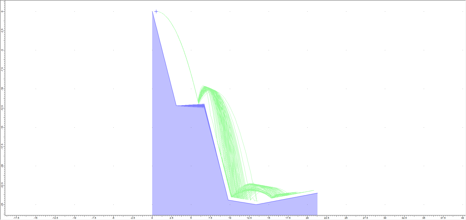
You should see the following.
As you can see, all rocks follow the same initial trajectory since there is zero variation in the seeder initial conditions. However, when they reach the second segment of the slope, many diverging paths are created due to the variation we applied to Vertex 3.
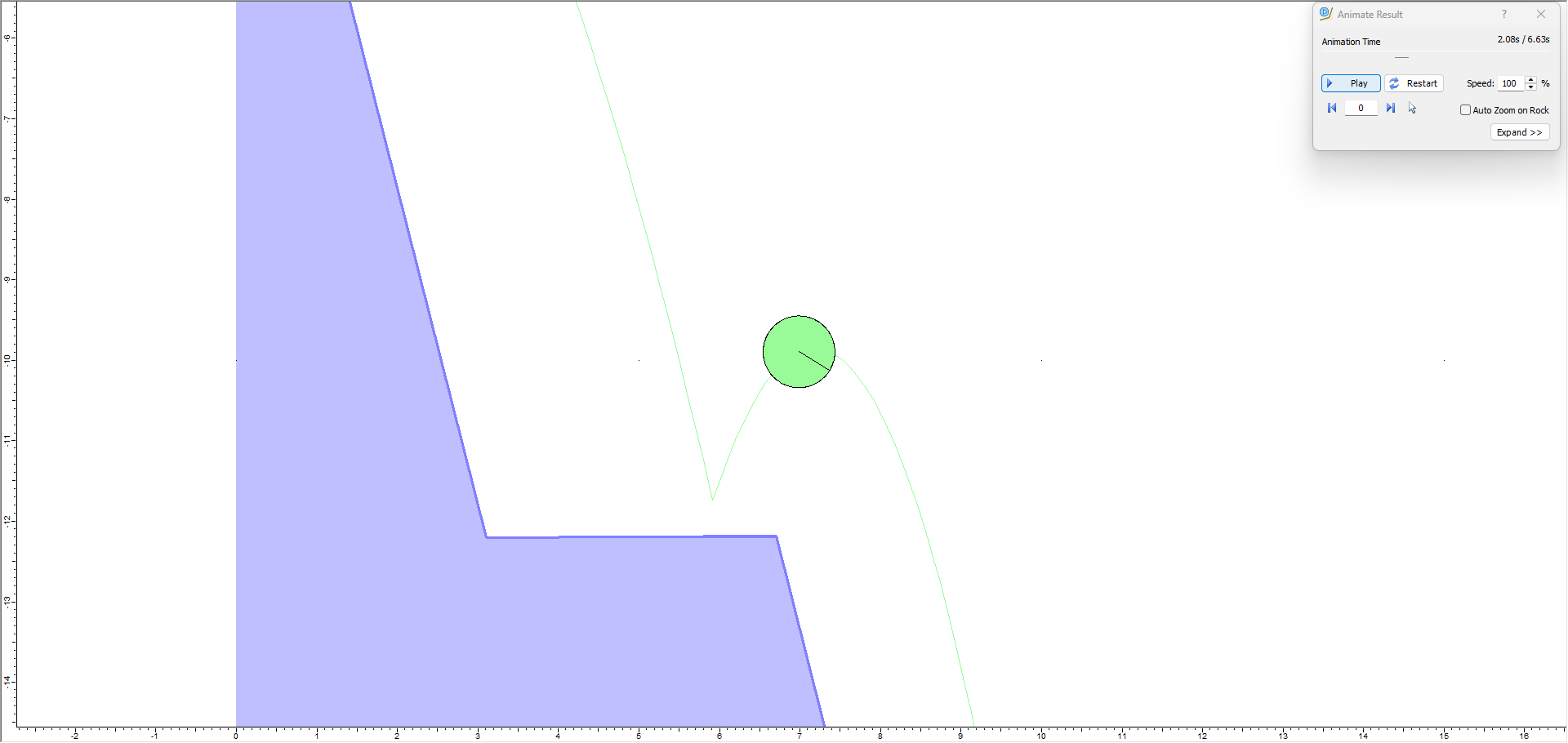
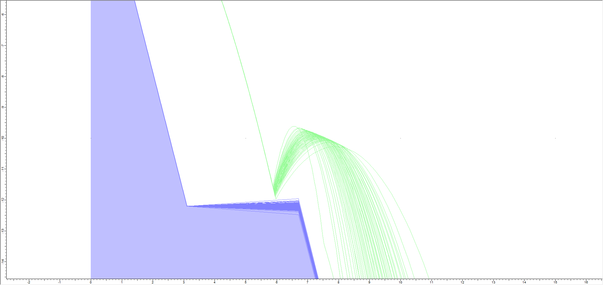
Let’s zoom in again to see what is going on. Use Zoom In (F4) to zoom in on the first bounce location of to left of Vertex 3 until your screen looks similar to the following. You may also find Zoom Window and Pan in the View menu useful.
This illustrates how the rocks can now bounce off slope segments above and below the mean slope segment orientation. The rock paths indicate the range of actual slope segments generated by the statistical variation we applied to Vertex 3. Effectively, a new slope is generated before each rock is thrown.
5.1 ANIMATE PATHS
Now we'll use the Animate Path option to view the rock fall.
Select Animate Path on the toolbar or the Results menu and zoom in if necessary.
In the Animate Result dialog, click through each rock path using the forward arrow beside the rock ID number.
NOTES:
Each time you view a new rock path, you can see the actual slope boundary segments generated for each rock throw.
For each rock throw, the coordinates of Vertex 3 are randomly generated according to the X and Y standard deviation you have entered. This results in the changing position of both boundary segments connected to vertex 3.
6.0 Sensitivity Analysis
When using vertex variation in RocFall2, you may find it useful to change the standard deviation of only one vertex at a time (leaving all other vertices with a standard deviation of 0). This will allow you to determine the sensitivity of the simulation to the location of that particular vertex. If you change the standard deviation of many vertices at once, it may be difficult to determine which vertex has the most effect on the results and which have very little effect.
7.0 Summary
This simple example shows how to model geometric variability of your slope coordinates using the vertex variation method. You can apply vertex variation to any or all vertices in a RocFall2 analysis in the Edit Boundary Coordinates dialog. In conjunction with statistical variation of other model parameters (rocks, initial conditions, material properties), you can simultaneously apply variability to any combination of rock fall input parameters.

 from the toolbar or the Analysis menu.
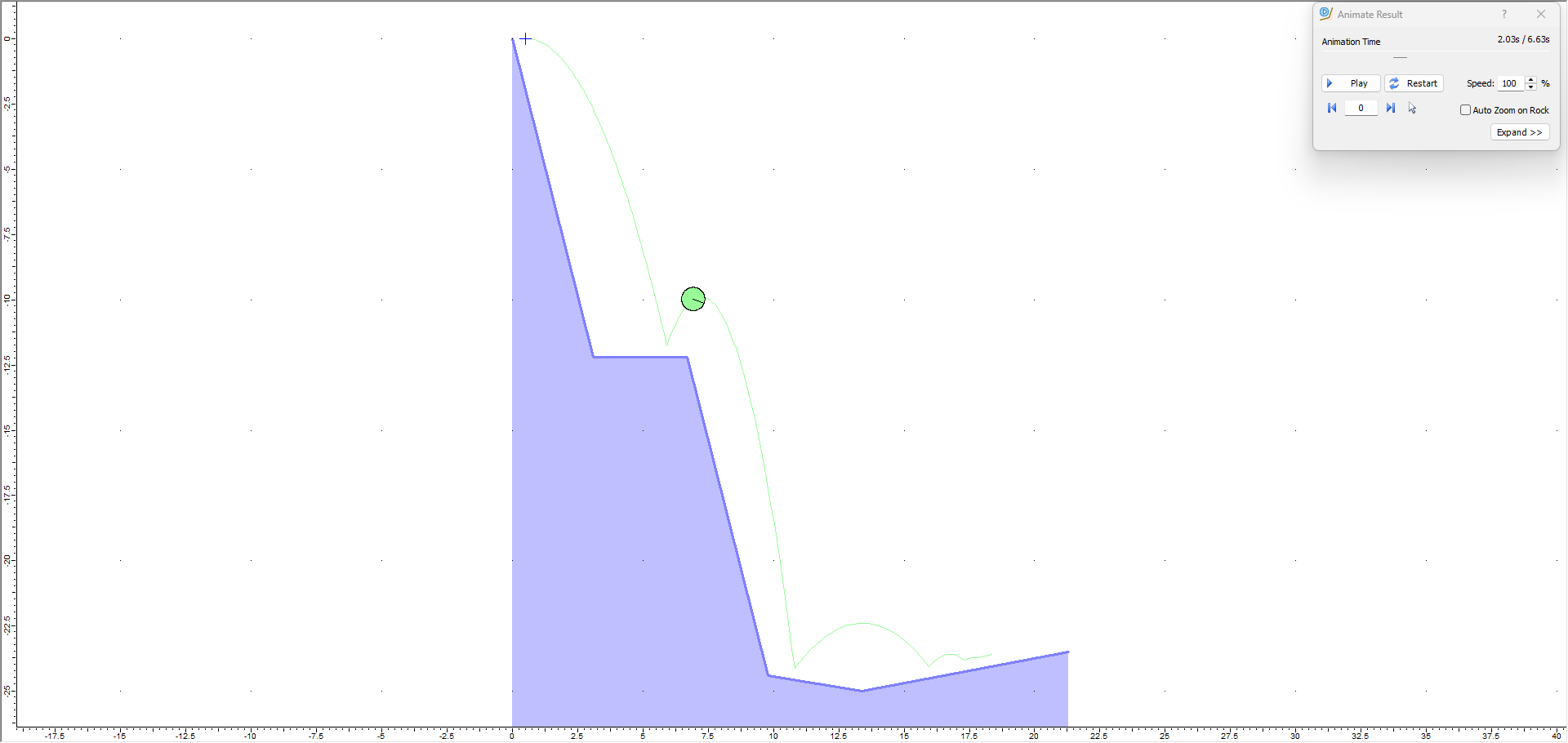
 on the toolbar.
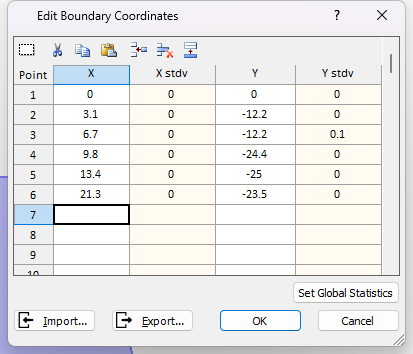
 on the toolbar or the Results menu and zoom in if necessary.