This tutorial will demonstrate the Barrier Sensitivity analysis option in RocFall2. Barrier Sensitivity allows you to automatically vary the location, height, angle, or capacity of rockfall barriers. Results are plotted as sensitivity plots, allowing you to determine the optimum location, height, angle, or capacity of rockfall barriers without the need to edit and re-compute multiple files. Output variables include rock energy, number of rocks impacting or passing a barrier, impact height, and velocity.
Topics Covered in this Tutorial:
X-Location, Height, Angle, and Capacity
Single input variable
Two input variables
Optimization based on energy, number of rocks, and impact height
Finished Product
The finished product of this tutorial can be found in the Tutorial 07 Barrier Sensitivity Analysis data file. All tutorial files installed with RocFall2 can be accessed by selecting File > Recent Folders > Tutorials Folder from the RocFall2 main menu.
2.0 Model
Let's start by opening the file for the tutorial.
SelectFile > Recent Folders > Tutorials Folder and open the Tutorial 07 initial file.
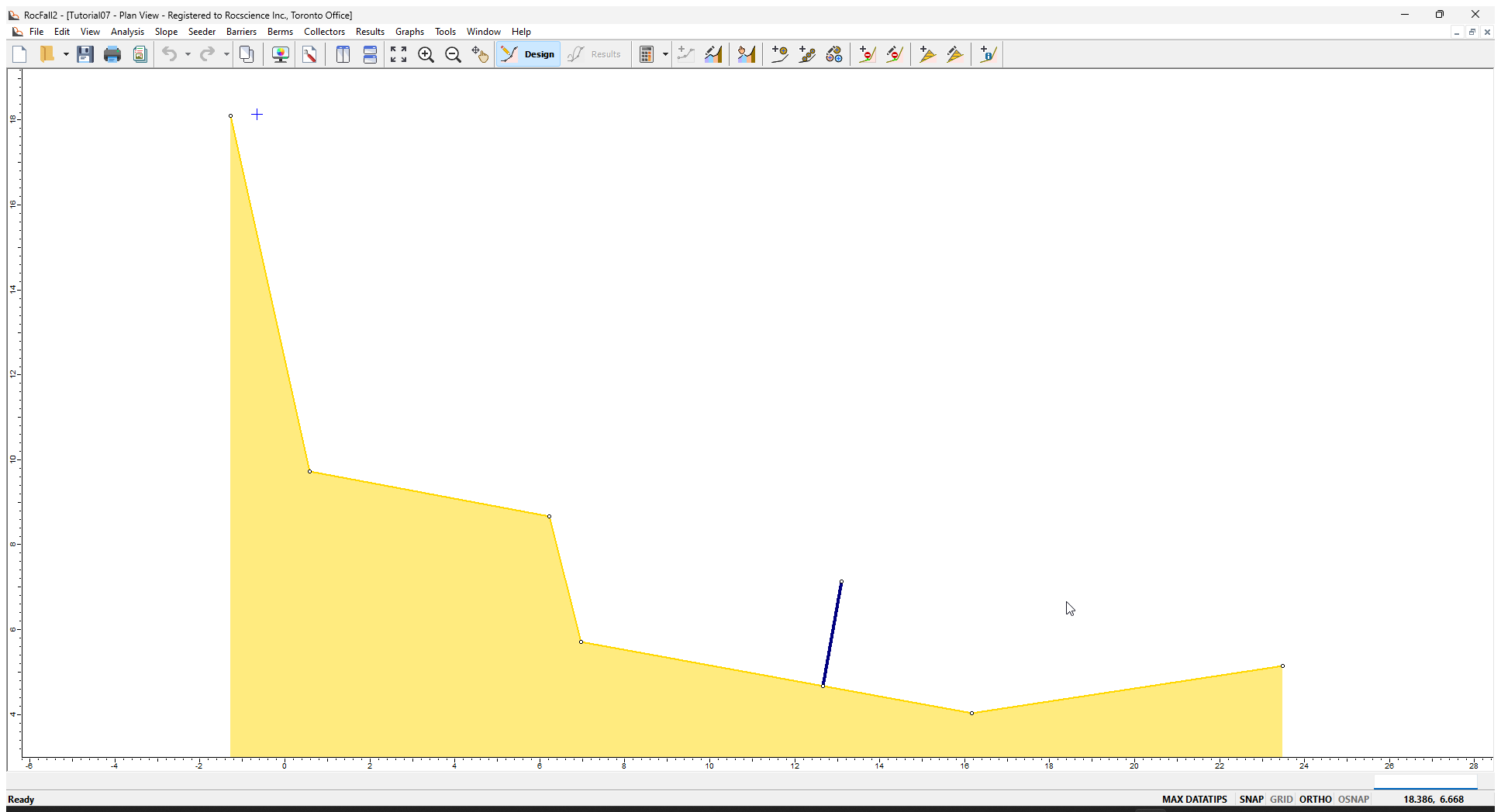
You should see the following model:
Initial RocFall2 model
The slope, barrier, rocks, and seeder have already been defined.
NOTE: Barrier sensitivity analysis can only be performed on ONE barrier at a time. If your model includes multiple barriers, you can still perform a barrier sensitivity analysis, but only ONE barrier can be chosen for sensitivity analysis. All other barriers will have fixed properties (X-Location, Inclination, Height, and Capacity).
2.0 Barrier Sensitivity Dialog
In order to carry out a barrier sensitivity analysis, you must first add a barrier to the model. In the above model, a single barrier has already been added. The Barrier Sensitivity can be opened by:
Selecting: Barriers > Barrier Sensitivity
Right-clicking on a barrier and select Barrier Sensitivity from the popup menu
You will then see the Barrier Sensitivity dialog:
In this dialog, you can choose:
Single Variable Analysis or Double Variable Analysis
The input Variable(s) for the analysis (X-Location, Length, Inclination, Capacity)
The Start/End values for the input Variable(s) and the number of Steps (i.e., the number of intervals between the values)
3.0 Single Variable Analysis
To start with, we'll demonstrate a Single Variable Analysis. With single variable analysis:
You choose ONE input variable (X-Location, Length, Inclination, Capacity)
After the analysis is run, you can plot one or more output variables versus the input variable on a sensitivity plot.
3.1 LOCATION SENSITIVITY
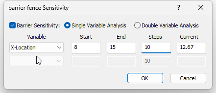
Let’s start with a sensitivity analysis of X-Location. This allows you to vary the barrier location by inputting the range of X-coordinates for the barrier. In the Barrier Sensitivity dialog:
Select Single Variable Analysis.
Set the following:
Variable = X-Location
Start = 8
End = 15
Steps = 10
Click OK.
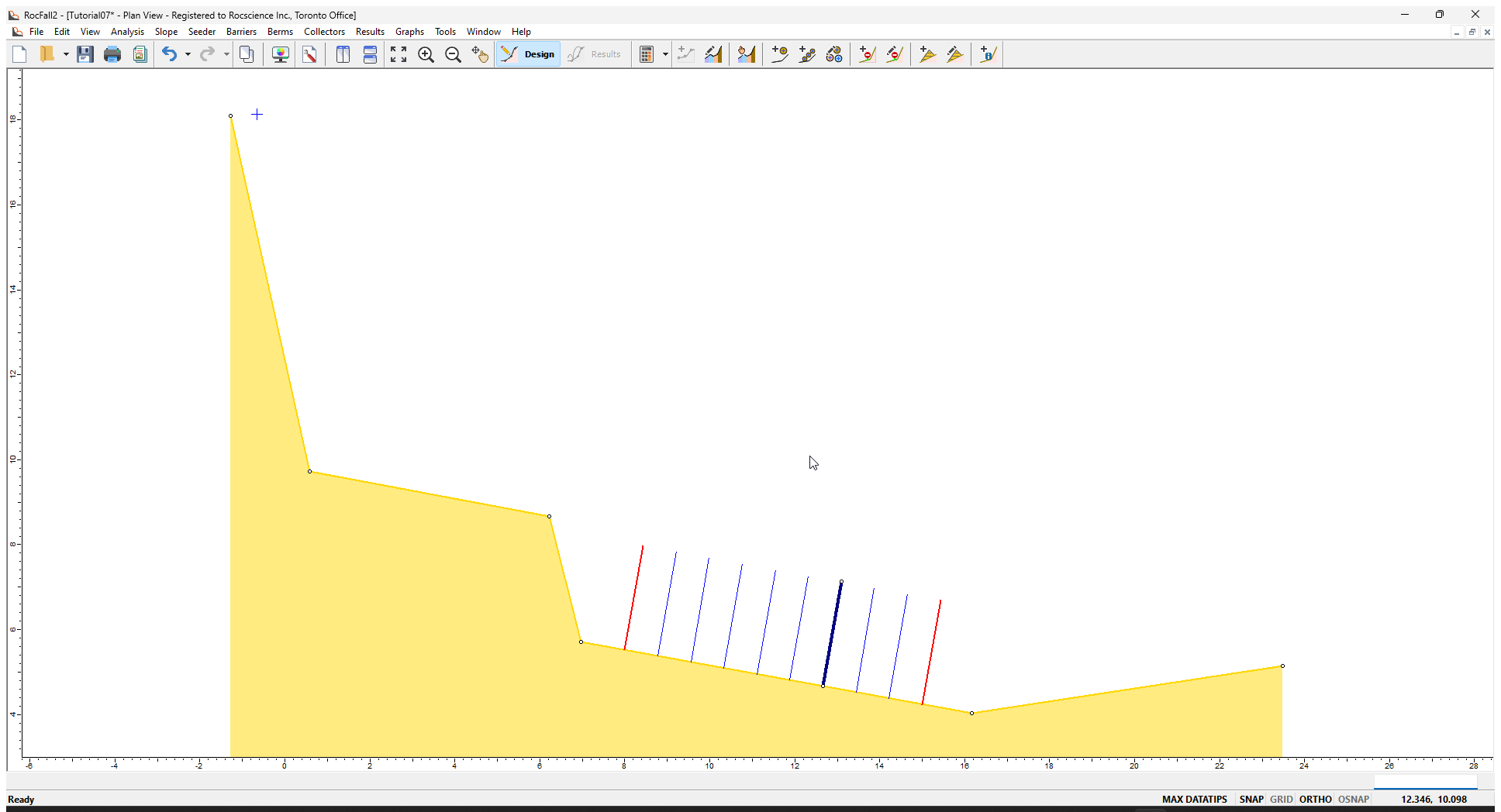
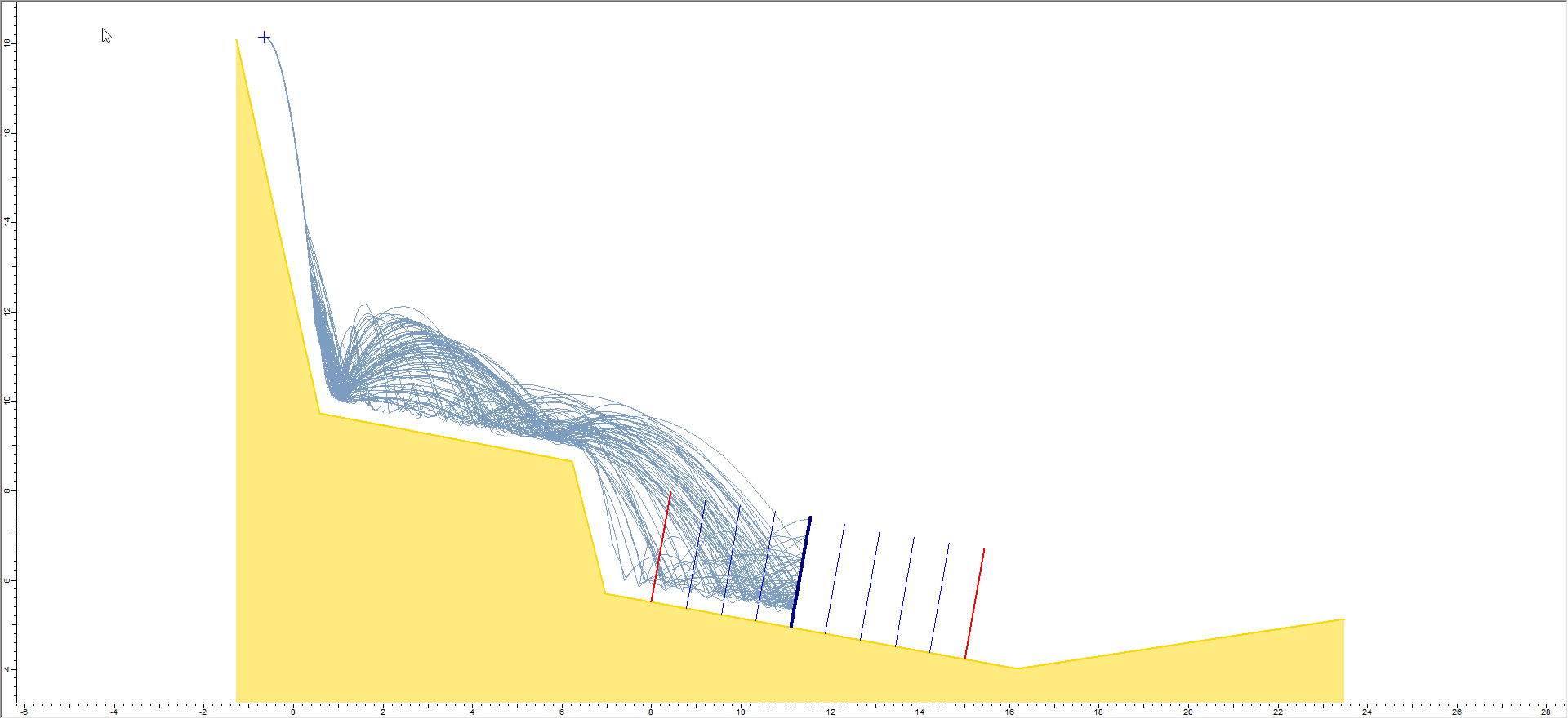
You should see the following, based on the range of X-Locations.
The min and max barrier locations are highlighted in red and the currently selected barrier is highlighted in dark blue. The locations correspond to the Start/End/Steps values entered for X-Location. The barrier Length and Inclination are constant since we are only varying the X-Location.
NOTE: Although the sensitivity display shows all barrier locations generated by the input, only ONE barrier is active (the currently selected barrier) for each analysis run.
Select the Compute option from the toolbar or the Analysis menu.
The sensitivity analysis is computed and you should see the following plot.
The above plot shows X-Location (horizontal axis) plotted against two output variables (maximum total energy and number of rock hits). These are the default output variables.
NOTE: If the plot is not automatically generated, then selectGraph > Graph Sensitivity and select output variables as discussed below.
3.2 SENSITIVITY ANALYSIS
A RocFall2 Barrier Sensitivity analysis means that the analysis is automatically repeated for EACH value of sensitivity input variable, in this case, the barrier X-Location. For each barrier location, the results are recorded and can be plotted on a sensitivity plot.
Let’s plot some additional output variables.
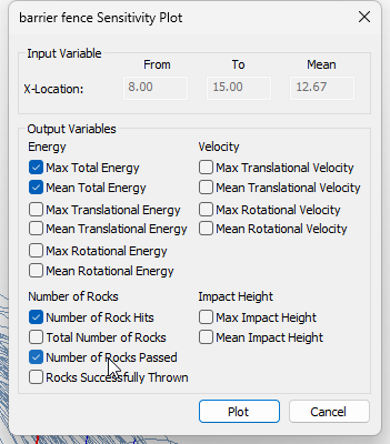
Select:Graph > Graph Sensitivity. You will see the Barrier Sensitivity Plot dialog.
NOTE: For Single Variable analysis, you will see the current input variable at the top of the dialog, and all available output variables. For output variables, you can select any number of variables to plot (e.g., one, two, three, or more).
Select Max Total Energy, Mean Total Energy, Number of Rock Hits, and Number of Rocks Passed for output variables.
Click OK.
You should see the following plot.
3.3 VIEWING DIFFERENT RESULT SETS
A very important property of the Barrier Sensitivity analysis is that you can obtain results for any individual analysis run (i.e., any value of input variable) by double-clicking the mouse on either:
A point on a Sensitivity Plot, or
A sensitivity barrier location on the model.
This automatically re-runs the analysis for that value of input variable, and the rock paths on the model are updated accordingly.
To demonstrate this:
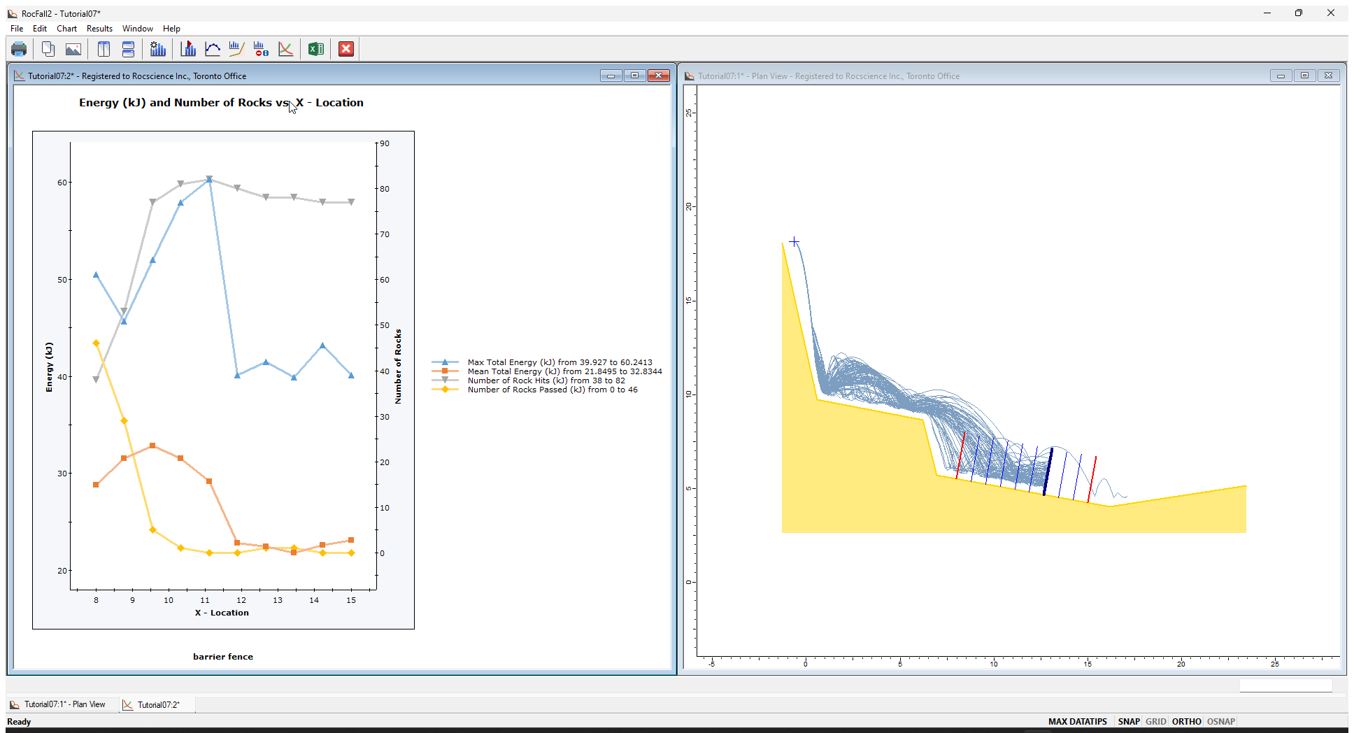
Select Window > Tile Vertically to vertically tile the views.
If you have two plot views open, close one and re-tile the views.
Double-click the mouse on:
The leftmost point on the sensitivity plot, or
The leftmost (first) sensitivity barrier in the model view.
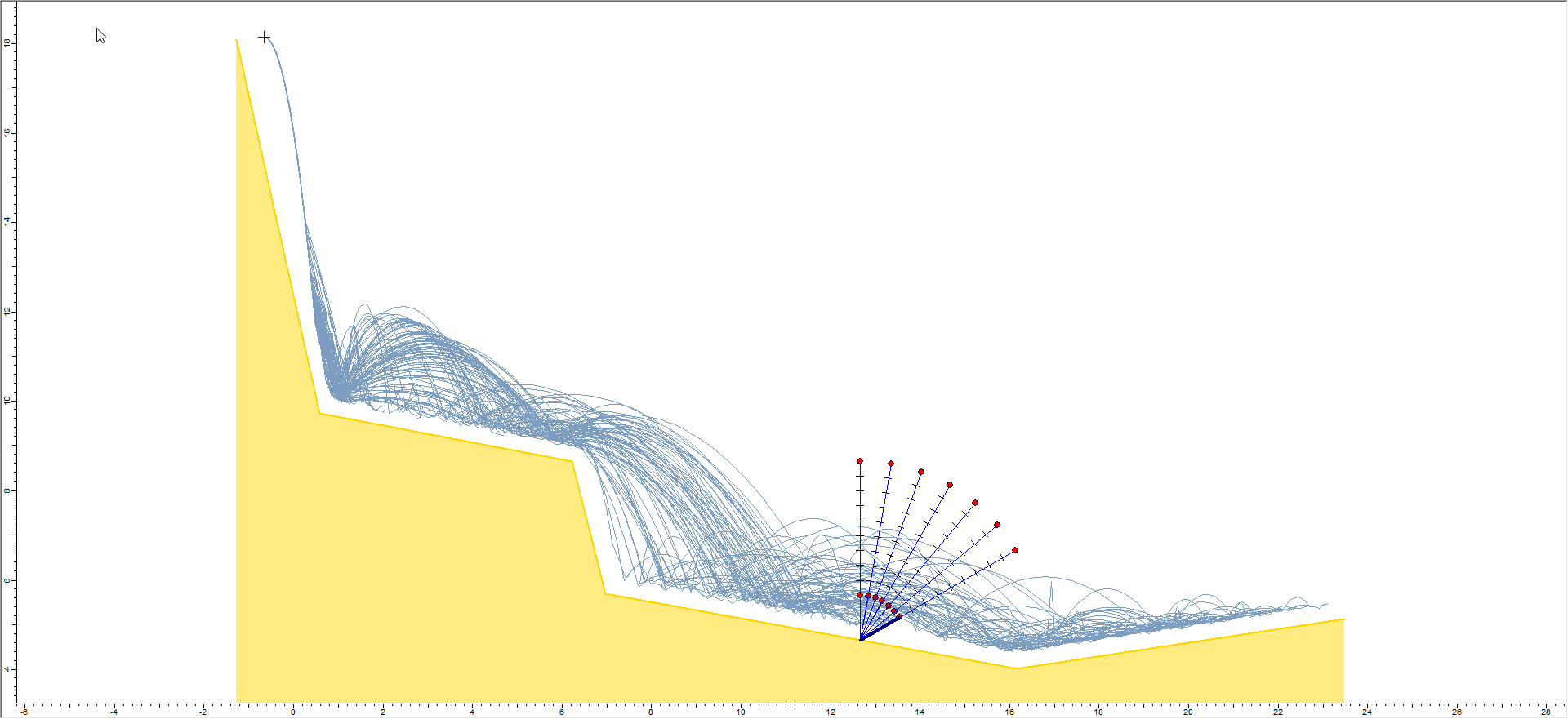
You will see that the analysis is re-computed and that the rock paths correspond to the selected barrier location, in this case the first barrier location. Notice that many rocks pass over the top of this first barrier. On the plot view, a vertical dotted line indicates the currently selected value of input variable.
Now double-click the mouse on successive barrier locations and notice how the rock paths are updated to correspond to the selected barrier.
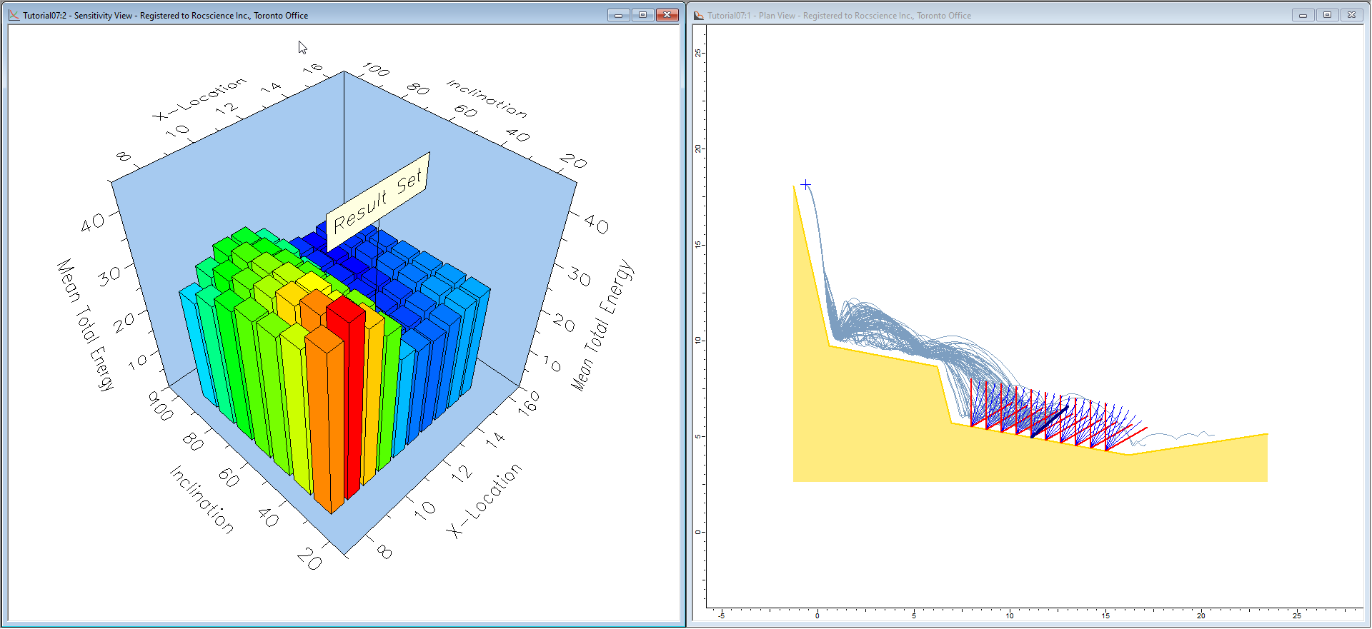
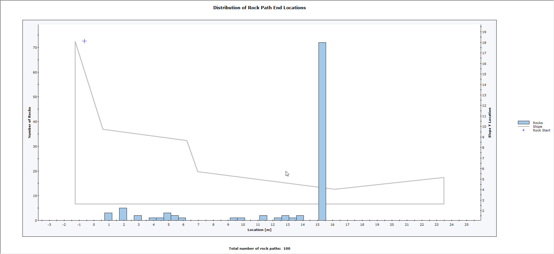
Another important thing to remember is that, once a particular barrier result set is being viewed, all other plotting options in RocFall2 (e.g., Graph Endpoints, Graph Data on Slope) will correspond to the current result set. For example, if you plot the Endpoint Location graph while the right-most sensitivity location is selected, you will see the following plot.
3.4 INCLINATION SENSITIVITY
Let’s now vary barrier Inclination (angle) at a constant location, height, and capacity:
Close all plots so only the slope model view is open.
Select Design on the toolbar to switch back to Design Mode.
Click Undo to go back to the default barrier.
Right-click on the currently selected barrier (dark blue) and select Barrier Sensitivity from the popup menu. The Barrier Sensitivity dialog appears.
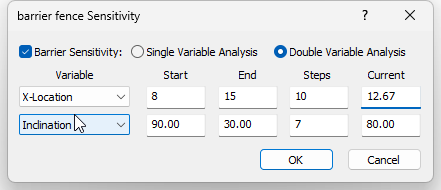
Set Variable = Inclination, Start = 90, End = 30, Steps = 7.
Click OK.
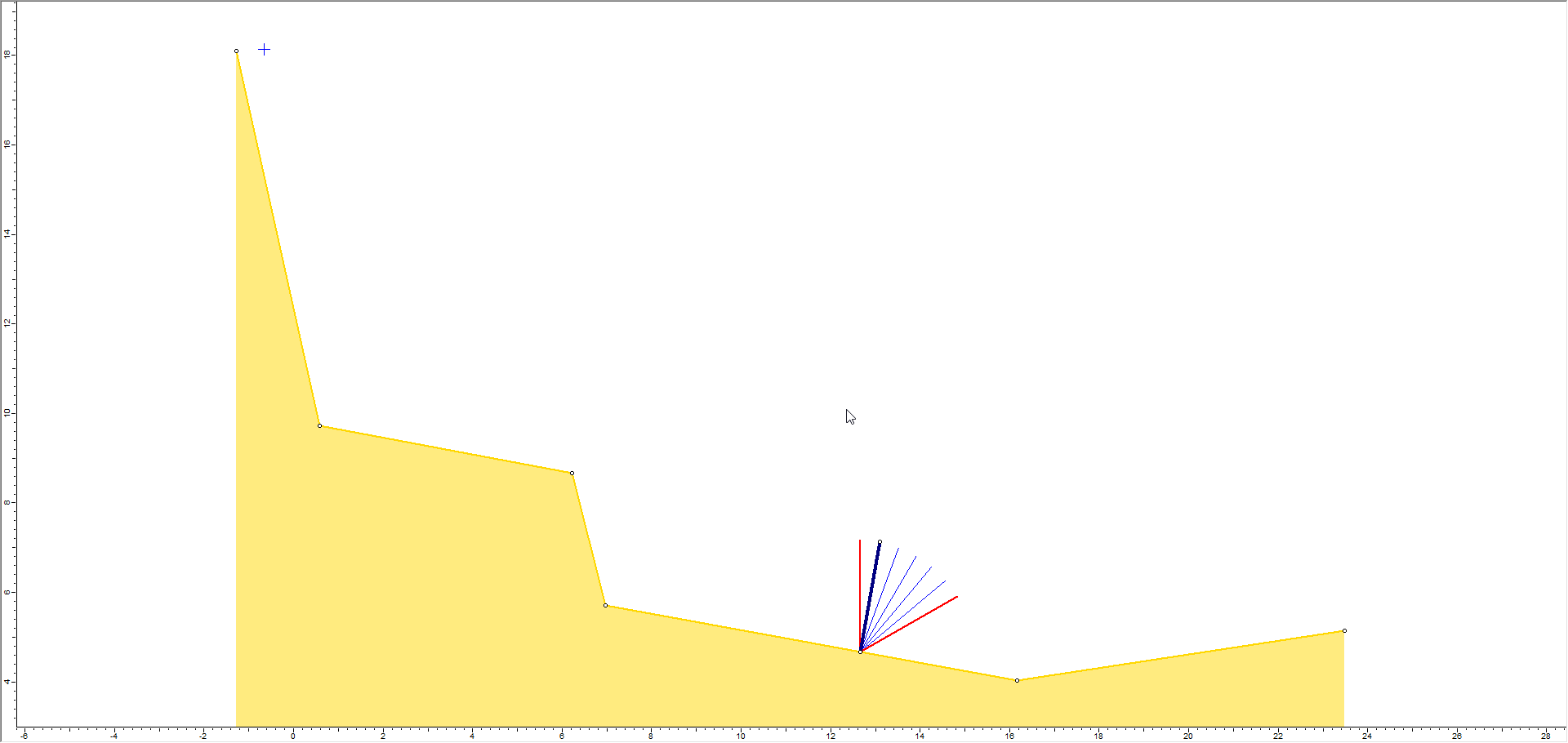
The model should look as follows. Note that the number of Steps = 7 gives 10 degree increments of inclination from 90 to 30.
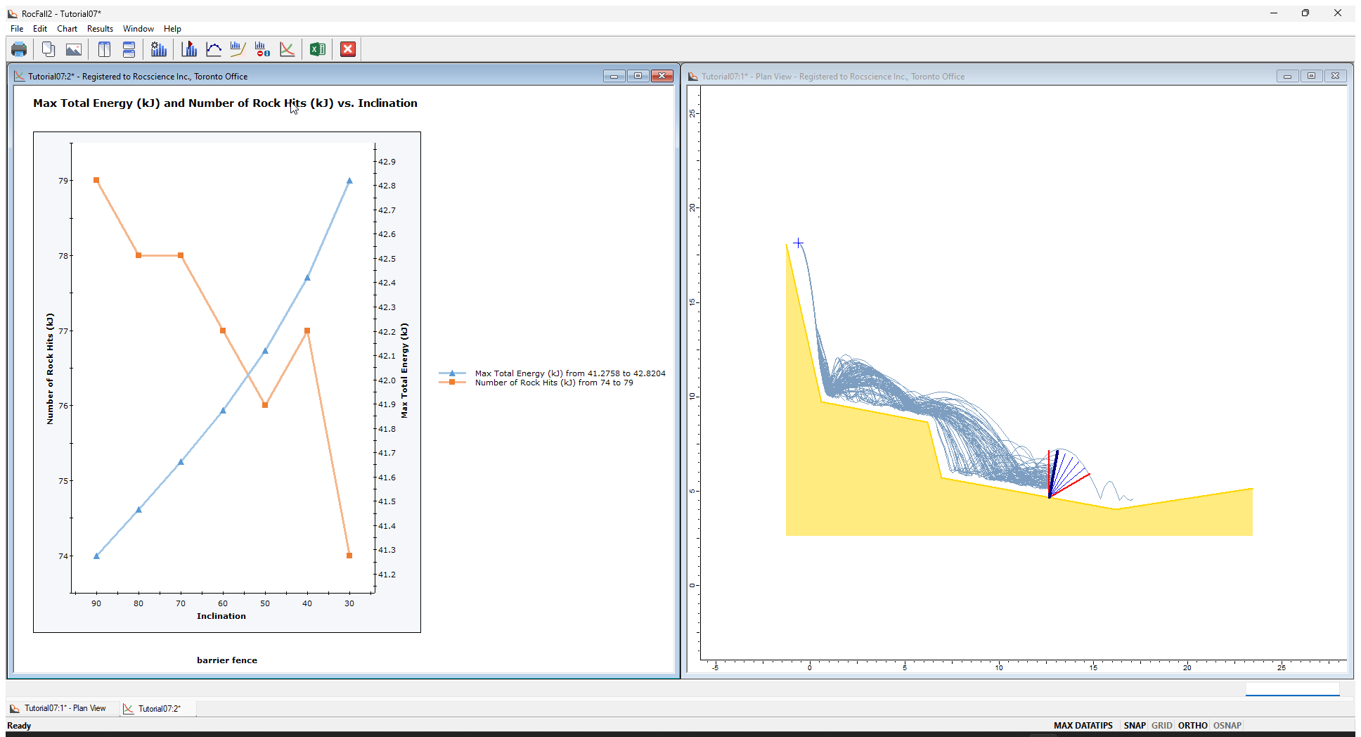
Select Compute and tile the views.
Now click on different data points on the sensitivity plot or on the sensitivity barriers on the slope model view to view the rock paths corresponding to the selected barrier inclination.
As we discussed with the location sensitivity, all other analysis results (e.g., Graph Endpoints, Graph Data on Slope) will correspond to the currently selected barrier.
3.5 HEIGHT SENSITIVITY
Let’s now vary barrier height at a constant X-Location, Inclination, and Capacity.
Close all plots so only the slope model view is open.
Select Design on the toolbar to switch back to Design Mode.
Click Undoto go back to the default barrier.
Right-click on the currently selected barrier (dark blue) and select Barrier Sensitivity from the popup menu.
Set Variable = Length, Start = 1.0, End = 4.0, Steps = 10.
Click OK.
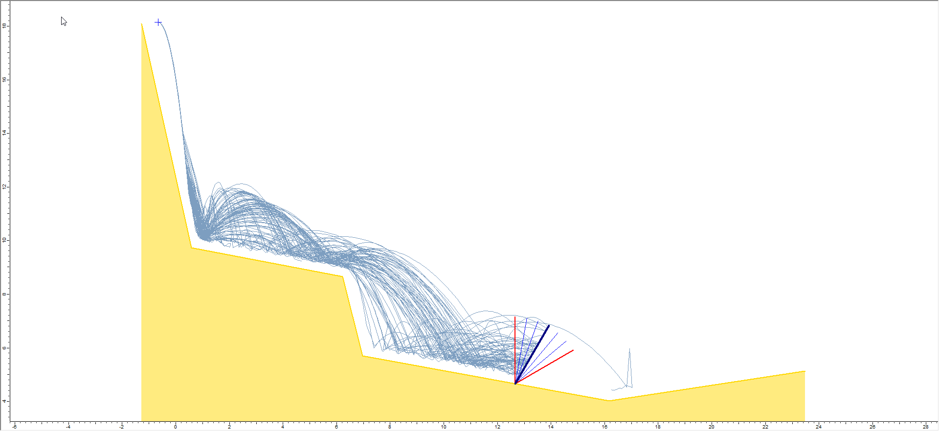
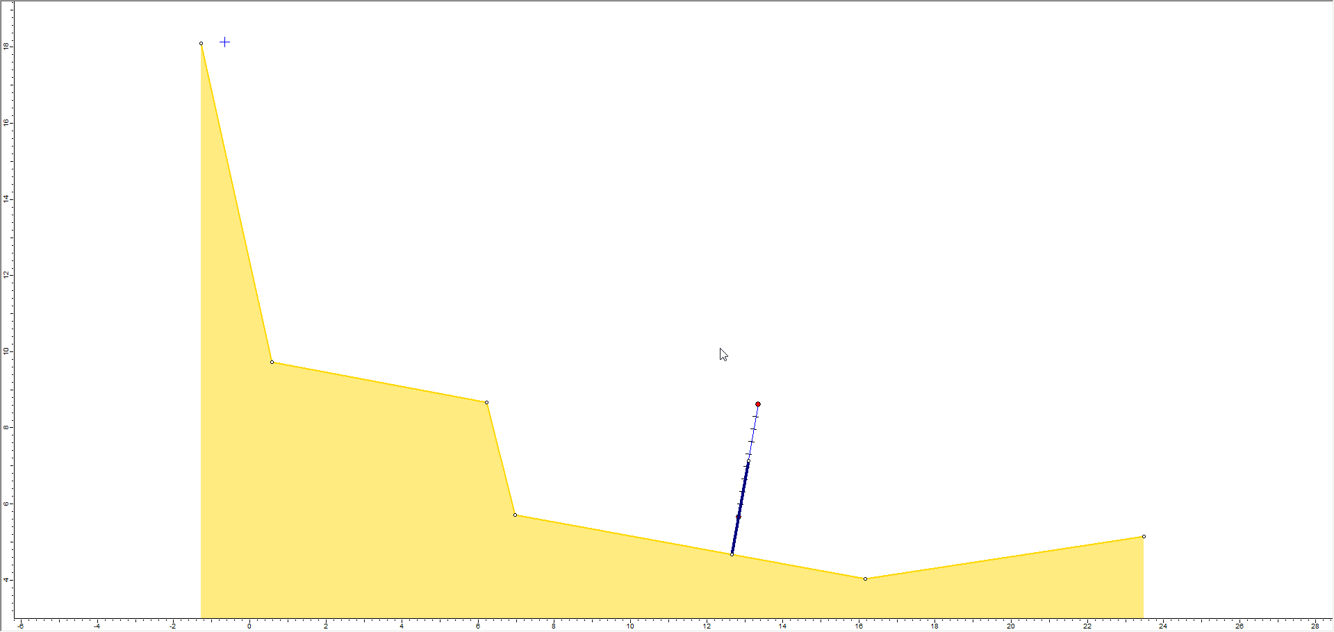
The model should look as follows:
Notice that Barrier Length Sensitivity is displayed as small red circles marking the min and max lengths, and discretizations along the length according to the number of Steps.
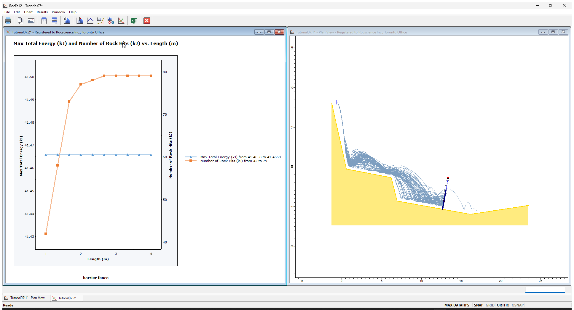
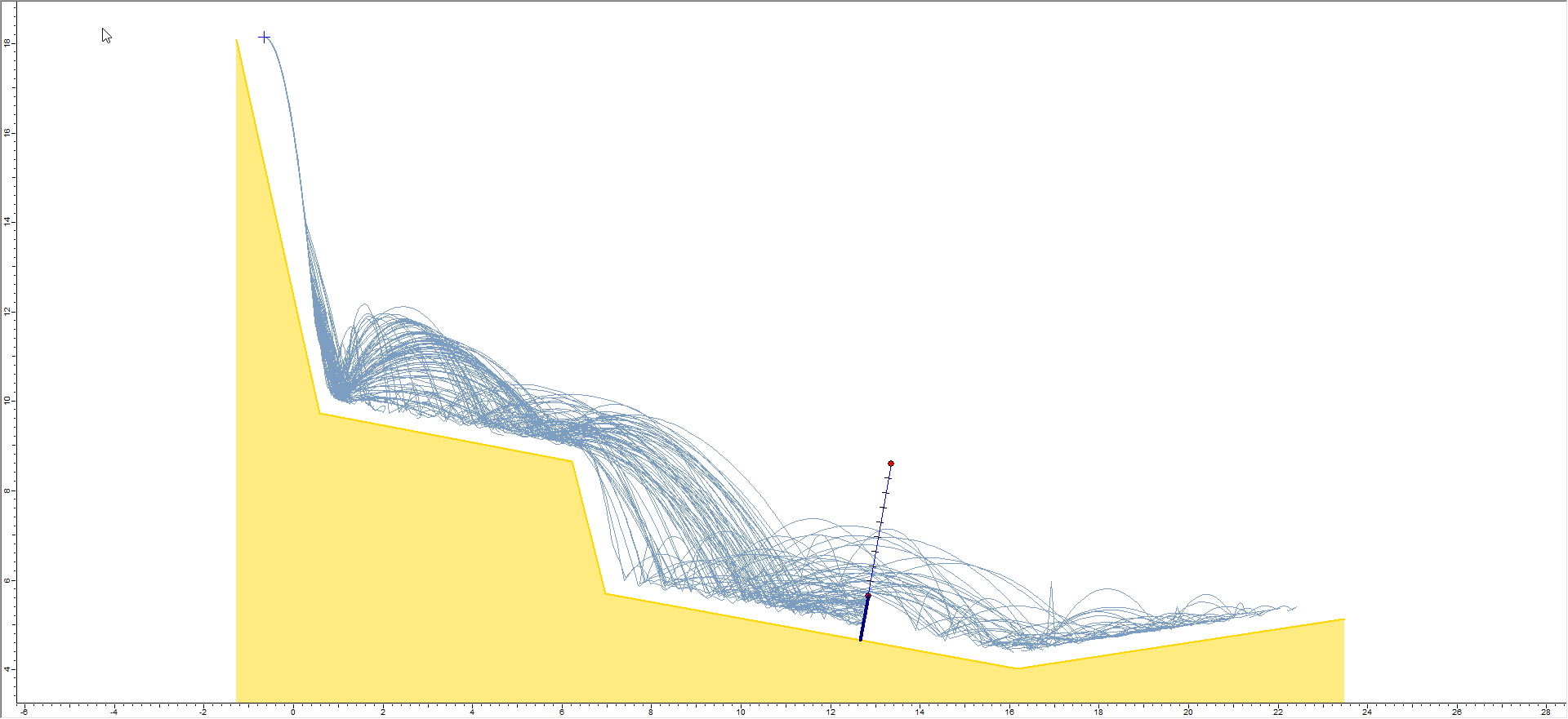
Select Compute and tile the views.
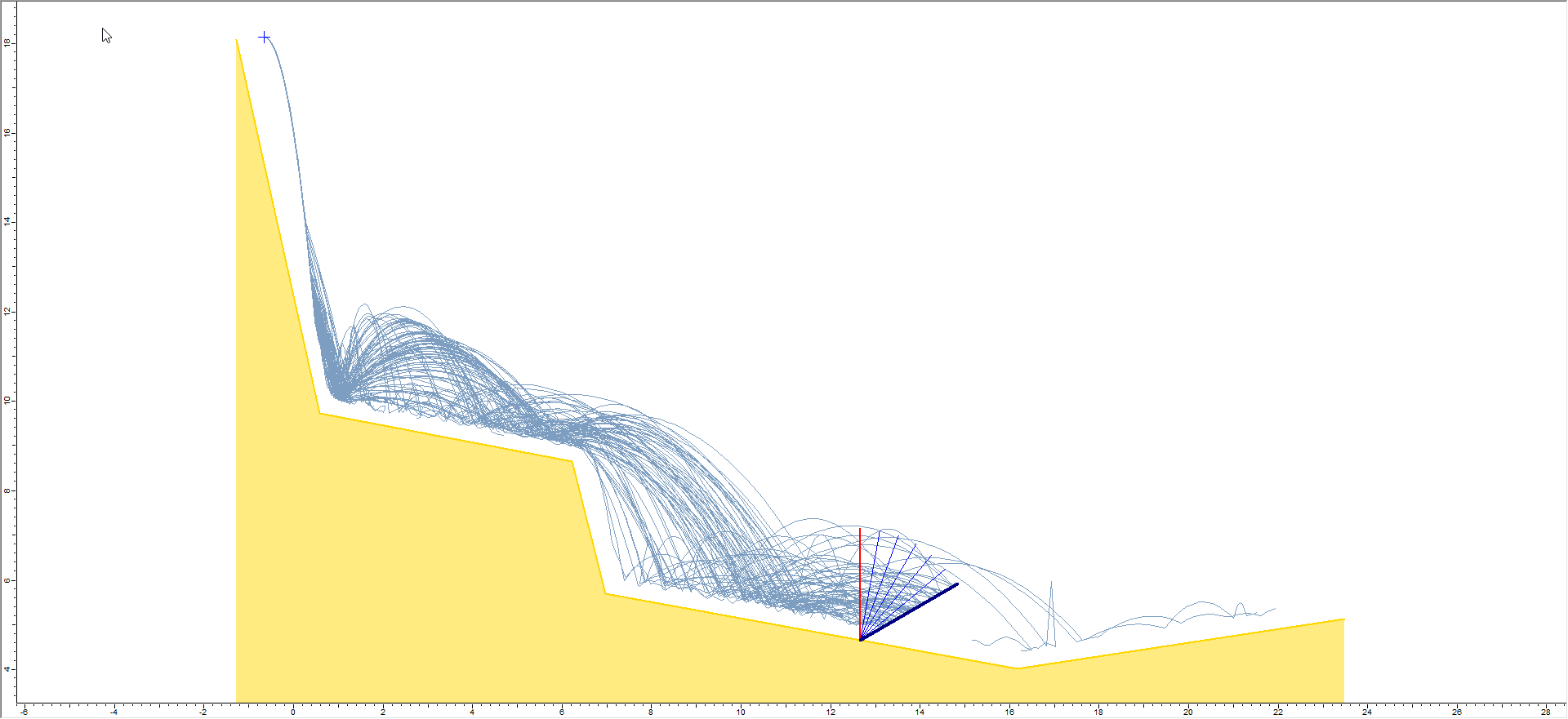
Now click on different data points on the sensitivity plot or on the sensitivity length discretizations on the slope model view to view the rock paths corresponding to the selected barrier length, for example the minimum length results shown below.
4.0 Double Variable Analysis
Now we will demonstrate Double Variable sensitivity analysis for barriers. Double variable sensitivity allows you to simultaneously vary two variables over user-defined ranges. For example:
Location and Inclination
Location and Length
Length and Inclination
Close the previous sensitivity plot so only the slope model view is open.
Select Design on the toolbar to switch back to Design Mode.
Click Undo to go back to the default barrier.
Right-click on the current barrier and select Edit > Barrier Properties in the popup menu.
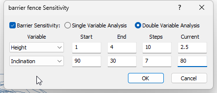
Select the Barrier Sensitivity check box.
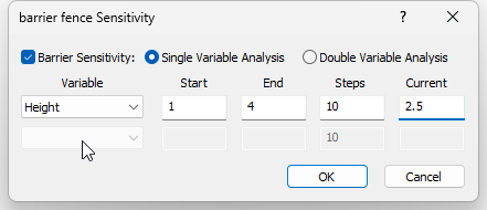
Select Double Variable Analysis.
Select Height and Inclination as the Variables and enter the values shown below.
Click OK.
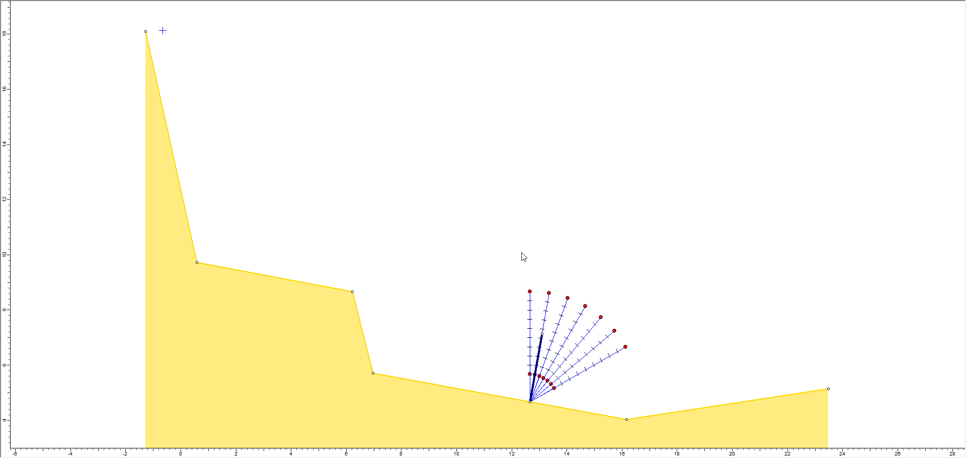
The model should appear as follows. Notice the barrier display now indicates the range of Inclination and Height values that will be generated during the analysis.
Select Compute.
A 3D plot should automatically be generated. The default output variable is Max Total Energy. In this case, the output variable Max Total Energy shows a constant value for nearly all values of Inclination and Length.
Let’s plot a different output variable.
Close the plot.
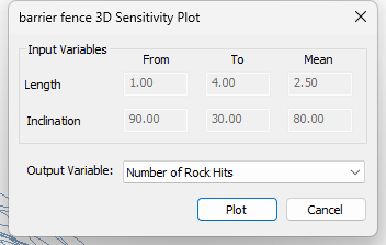
Select Graphs > Graph Sensitivity. You should see the Barrier 3D Sensitivity Plot dialog. Note that for Double Variable analysis, the dialog indicates the two Input Variables and you can select only one Output Variable.
Choose Number of Rock Hits as the Output Variable.
Click Plot.
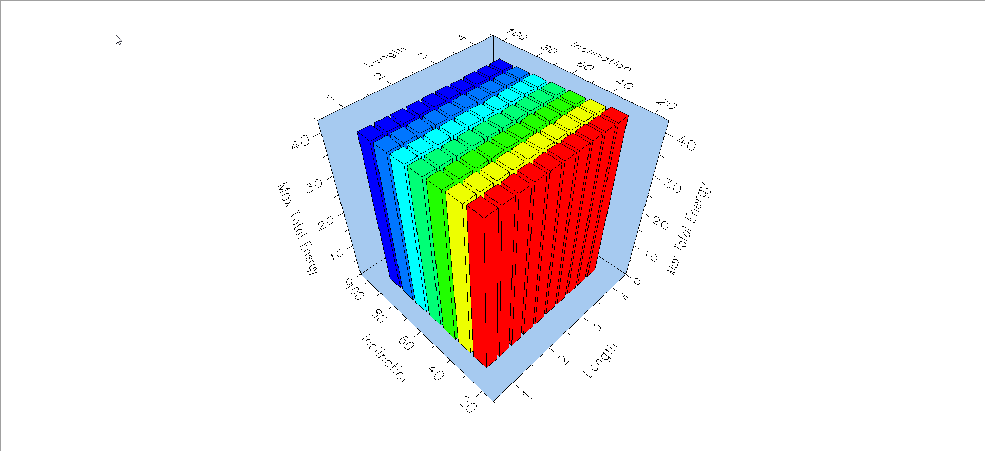
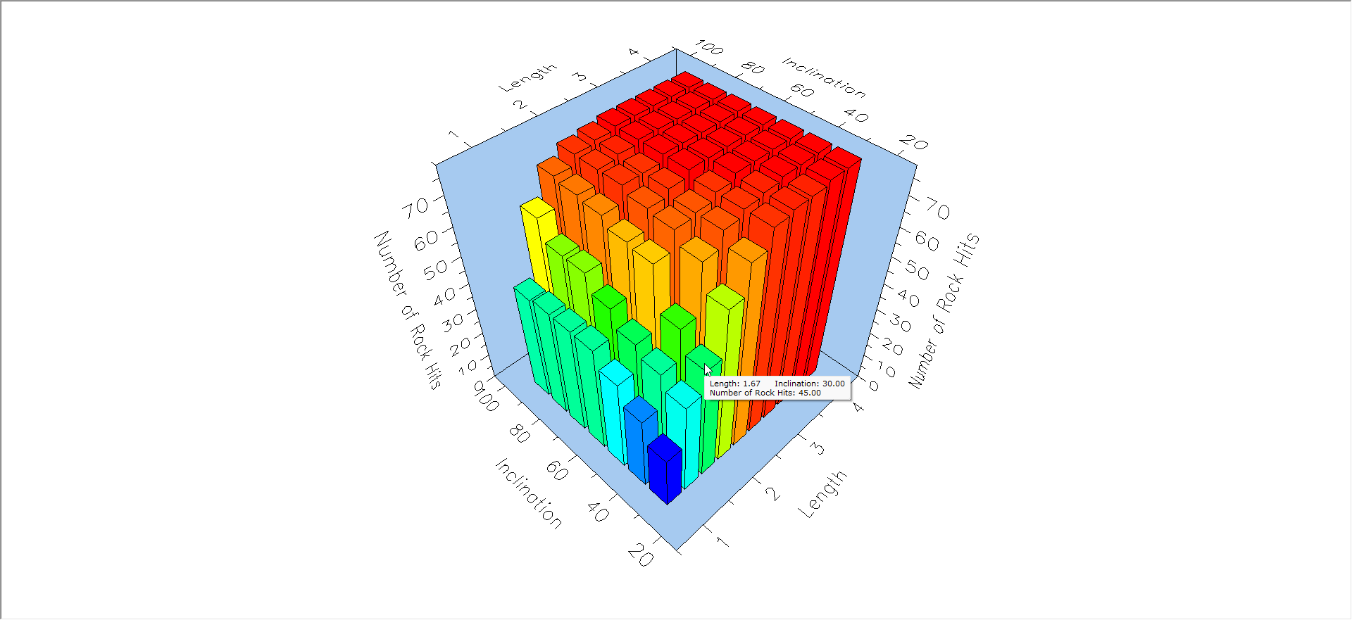
The 3D plot should look as follows:
For double variable analysis, the same functionality exists as for single variable analysis. You can click on the 3D plot or on the barriers on the model to obtain the rock path results corresponding to that combination of input variables. For example, on the above 3D plot, the minimum number of rock hits occurs at the smallest values of length and inclination.
Double-click on the blue histogram bar at this minimum value.
You should see the following result on the model.
As expected, the shortest barrier with the flattest inclination has the minimum number of rock hits for this example. Conversely, if you plot the Number of Rocks Passed, this barrier will have the Maximum number of rocks passed.
4.1 LENGTH AND INCLINATION
Let’s plot a different combination of variables.
Close all 3D plots so that only the slope model view is open.
Select Design on the toolbar to return to Design Mode.
Click Undo to go back to the default barrier.
Right-click on the currently selected barrier (dark blue) and select Barrier Sensitivity from the popup menu.
Select X-Location and Inclination as the Variables and enter the ranges shown below.
Click OK.
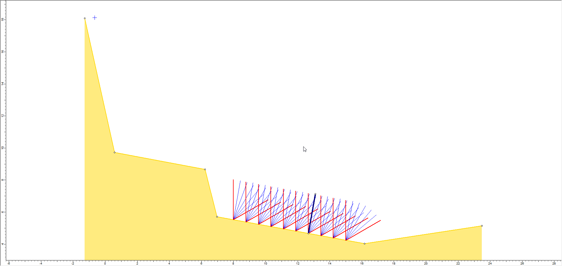
You should see the following:
Select Compute.
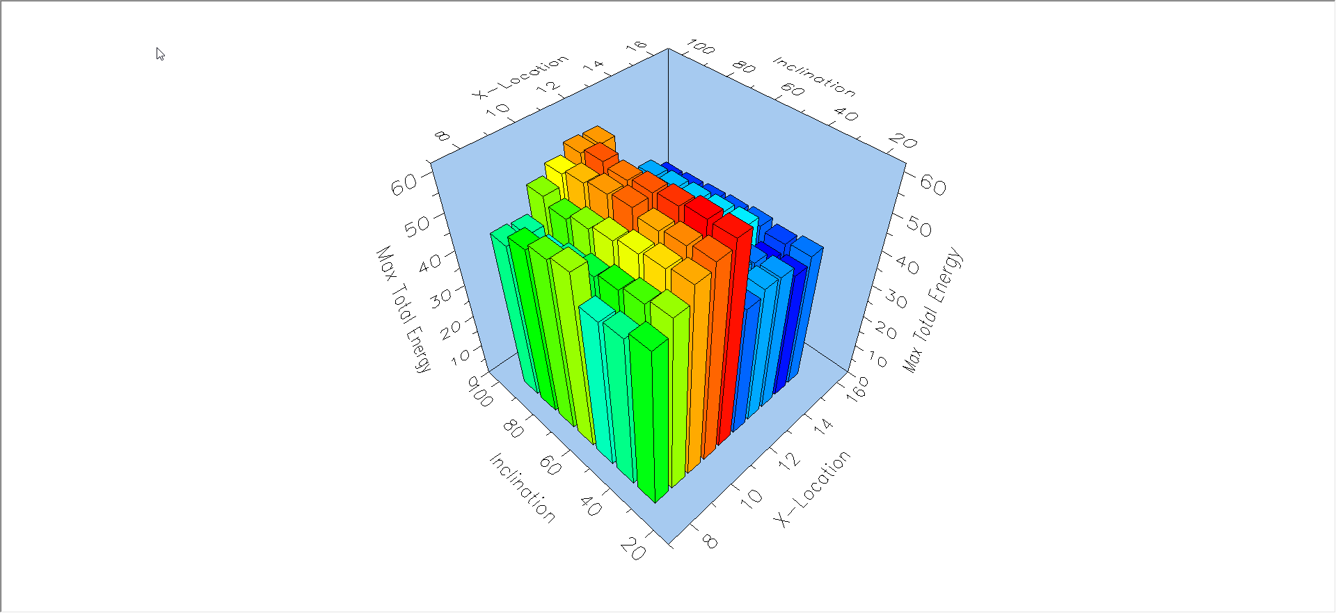
The compute dialog indicates the progress of the sensitivity analysis and each individual analysis run (rock throws). When the compute is finished, the following plot should be automatically generated.
In this case, the Maximum Total Energy is quite variable over the range of the two input variables. Tile the views.
4.2 DISPLAY RESULTS FOR MINIMUM OR MAXIMUM VALUES
Another useful feature of 3D plots is that you can automatically locate the minimum or maximum values of the output variable with a right-click shortcut.
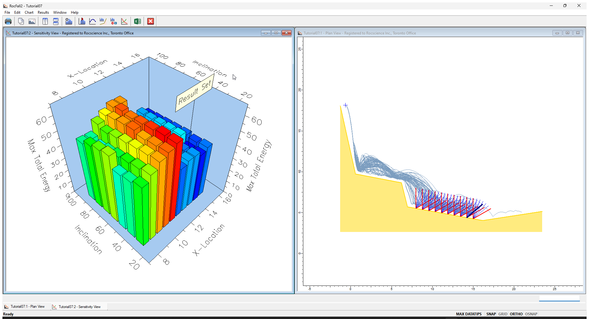
Right-click on the 3D plot, and select Pick Result Set to Minimize Value from the popup menu. You should see the following rock path results.
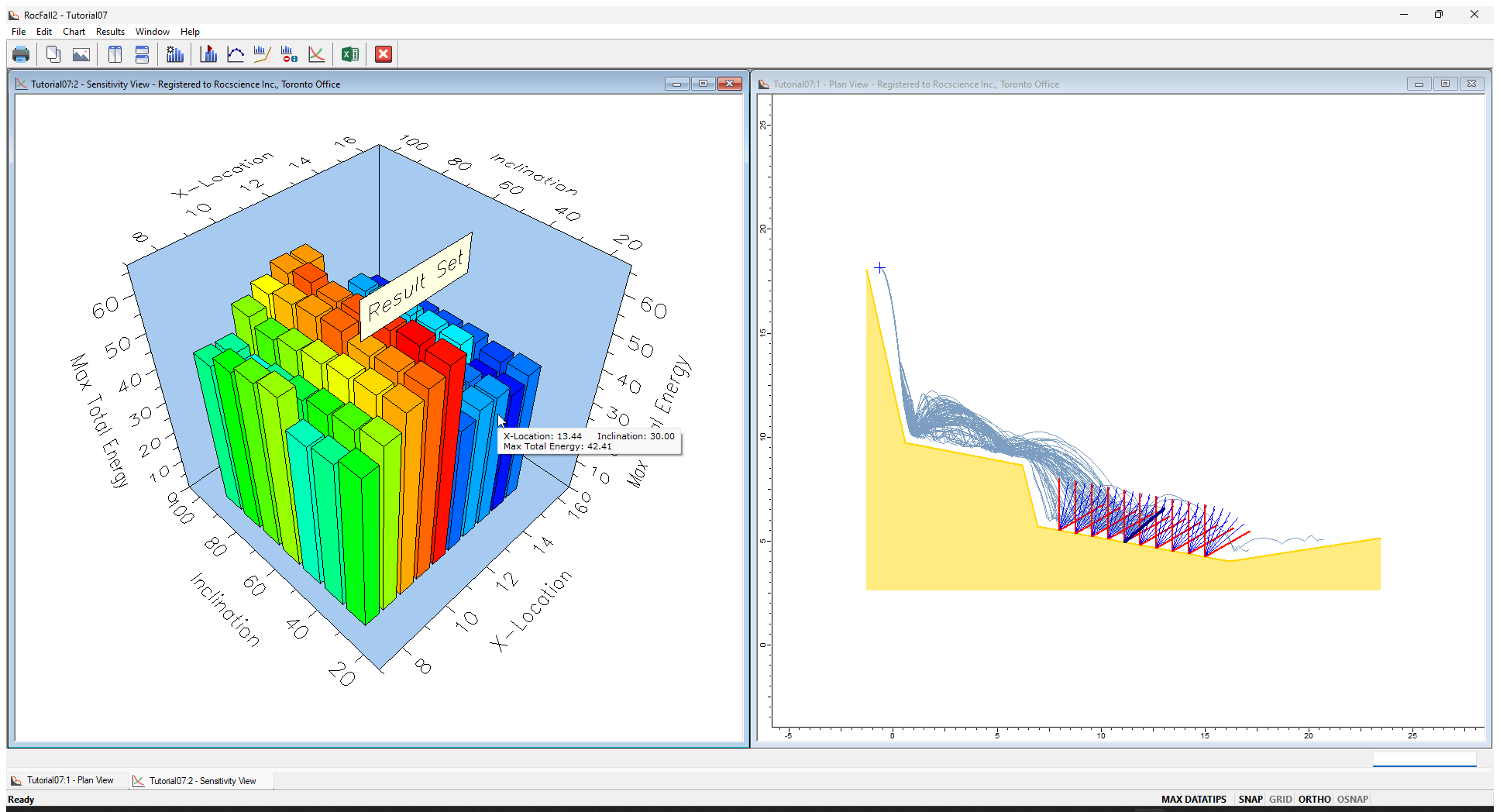
Now right-click on the 3D plot and select Pick Result Set to Maximize Value from the popup menu. You should see the following rock path results:
4.3 MEAN TOTAL ENERGY
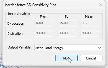
You are encouraged to experiment with the Barrier Sensitivity analysis and plotting options. For example, using the Location and Inclination example above, plot the Mean Total Energy on a barrier and compare results with the Max Total Energy Plots.
Use the right-click shortcut to display results for the Minimum and Maximum values of Mean Total Energy (right click on the barrier and select Graph Barrier Sensitivity). Notice that the results are different compared to the Max Total Energy results. In general, Mean Total Energy results may be a better variable to optimize as it considers the average of all rock hits on a barrier, whereas the Max Total Energy usually represents only a single rock, which may possibly represent a statistical outlier value.
4.4 BARRIER CAPACITY
In this tutorial, we have not demonstrated sensitivity analysis using Barrier Capacity as an input variable. This is left as an optional exercise.
Note that there is currently no graphical representation of the barrier capacity in the model view for a barrier sensitivity analysis. A text label will indicate the values of the capacity range, but you cannot double click in the model view to select the barrier capacity. You can click in the plot views to select barrier capacity. As you vary barrier capacity, rocks may either stop at a barrier or pass through a barrier, depending on the capacity, therefore this may affect the number of rocks which can pass a barrier, by travelling over or through the barrier.
 option from the toolbar or the Analysis menu.
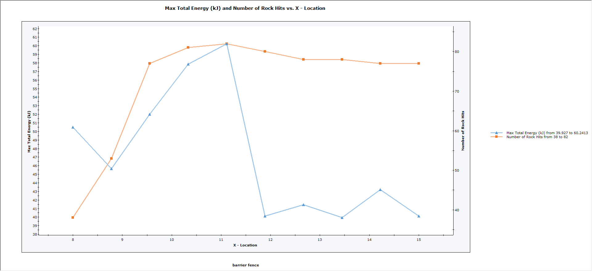
 NOTE: For Single Variable analysis, you will see the current input variable at the top of the dialog, and all available output variables. For output variables, you can select any number of variables to plot (e.g., one, two, three, or more).
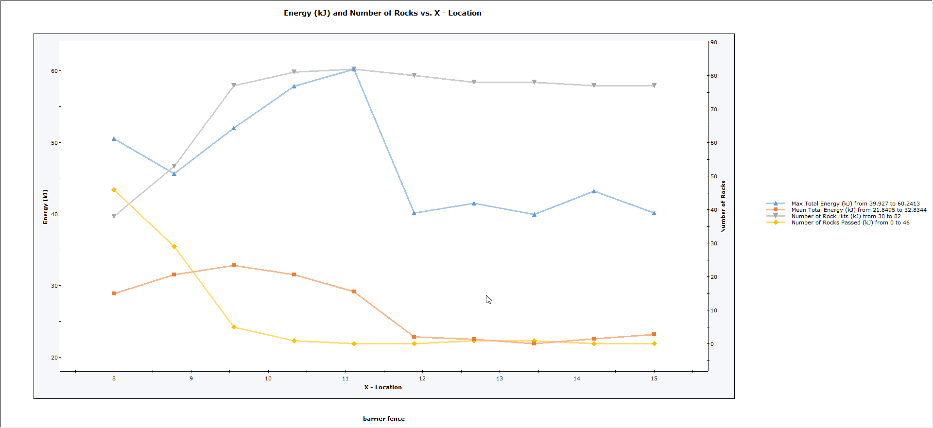

 to go back to the default barrier.
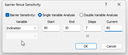

 on the toolbar to switch back to Design Mode.