21 - Rapid CPT Data Import
1.0 Introduction
In Settle3, Rapid CPT data import allows users to import multiple CPT data from data forensics. After entering Log-in information from the database, users can import multiple CPT from the cloud server and import multiple CPT data in Settle3. These CPT data can be used to analyze multiple CPT analysis, and plot soil profile as well as SBT (Soil Behavior Type) graph.
In this tutorial, we will show how this procedure is made by importing the data from data forensics. If you do not have access to the cloud server, you can still follow our tutorial with the files in the tutorial folder which contains .txt file.
Topics Covered in this Tutorial:
- CPT analysis
- Multiple CPT Data import
- Multiple CPT data analysis
Finished file:
The finished file of this tutorial can be found in the Tutorial 21 Rapid CPT Data Import.s3z file. All tutorial files installed with Settle3 can be accessed by selecting File > Recent Folders > Tutorials Folder from the Settle3 main menu.
2.0 Model
2.1 Project Settings
- Select Home > Project Settings
 (CTRL + J) to open the Project Settings dialog.
 - In the General tab, make sure the Stress Units are set to Metric, stress as kPa and the Settlement Units are set to Meters.
- In the Cone Penetration Test (CPT) tab, make sure to check the box for CPT Analysis. We will use the Robertson 1986 CPT Classification with default values for atmospheric pressure (kPa), Net Area Ratio, and Cone Factor.
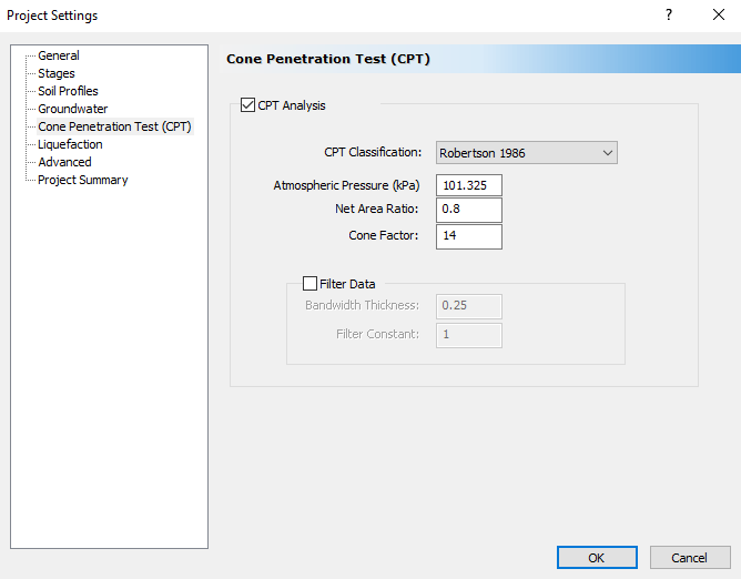
- Click OK.
3.0 Import Multiple CPT Data from Data Forensics
We will now import multiple CPT data from data forensics.
- Select CPT > Add CPT
 .
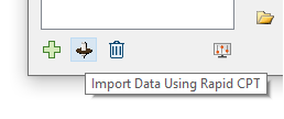
. - Add multiple CPT by selecting the Import Data Using Rapid CPT button at the bottom left.
- You will be prompted with log-in information for Data forensics. Enter your credentials below:
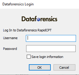
- If you do not have login information for Dataforensics Rapid CTP, we will simulate the process for this tutorial purposes.
Please enter:
- Username: tutorial
- Password: tutorial
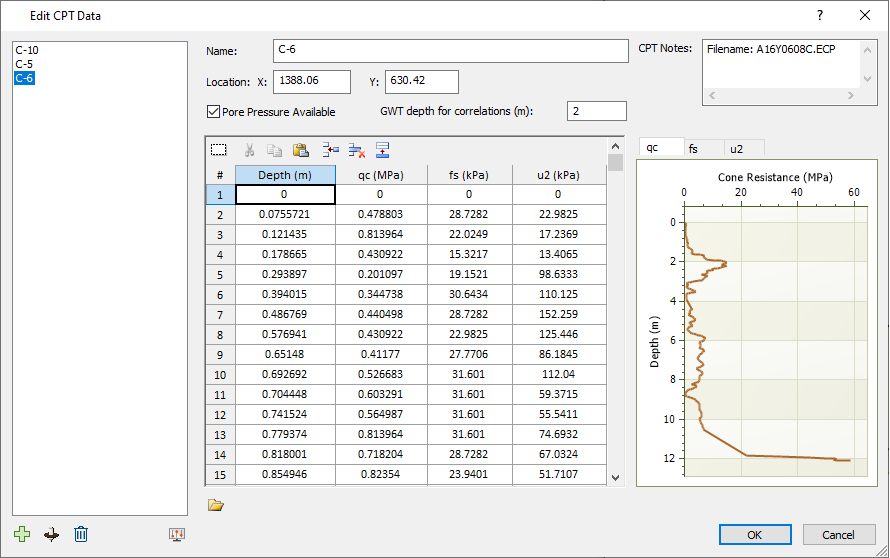
C-5: (X = 1346.56, Y = 380.52)
C-10: (X = 1288.06, Y = 530.42)
C-6: (X = 1388.06, Y = 630.42)
Otherwise, if you keep the values as they are, you will get a warning message for large coordinates for importing those coordinates due to issues in displaying the model on 2D and 3D views with large coordinates.
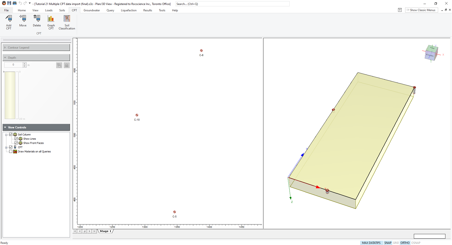
4.0 CPT Analysis Result
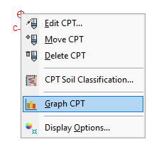
After multiple CPT data are imported, you can check the CPT analysis for each data by:
- Right-clicking on the data and selecting Graph CPT
 .
.
When you graph CPT plot, you will see the result as shown below for the first data.
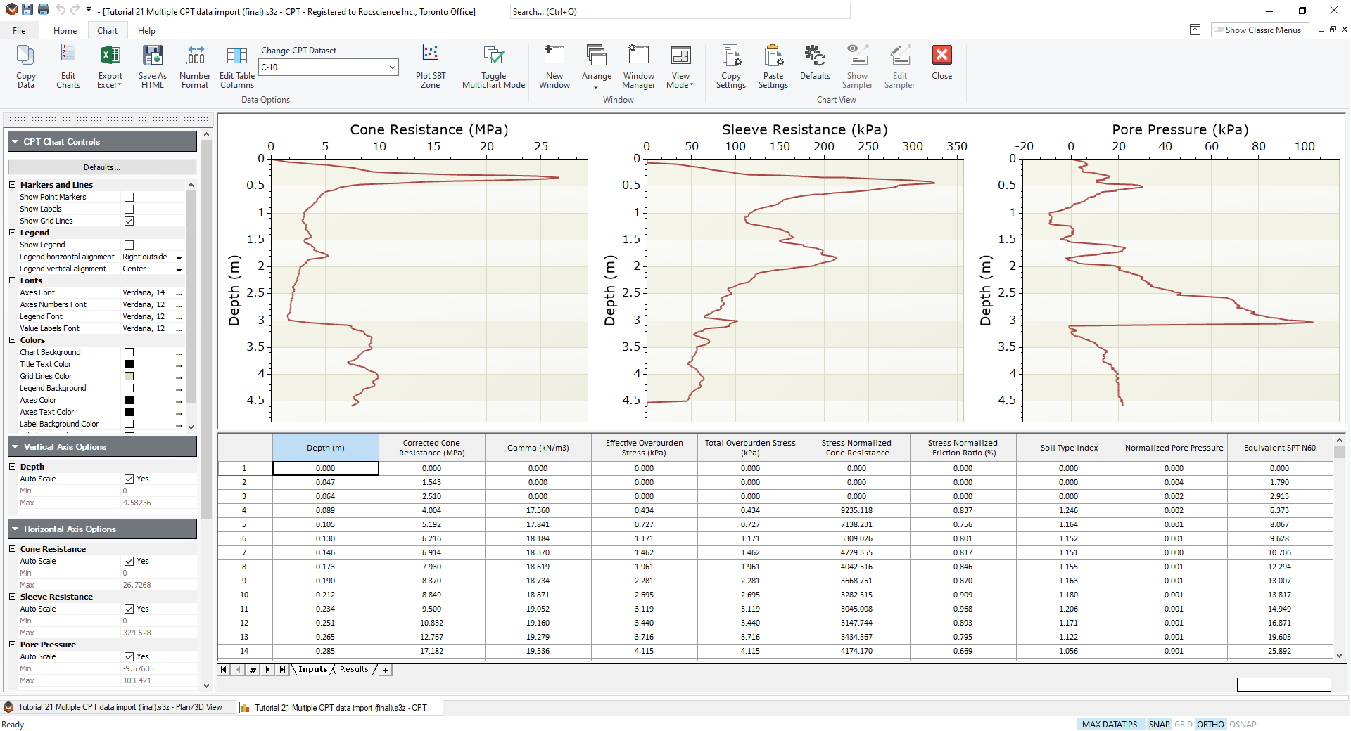
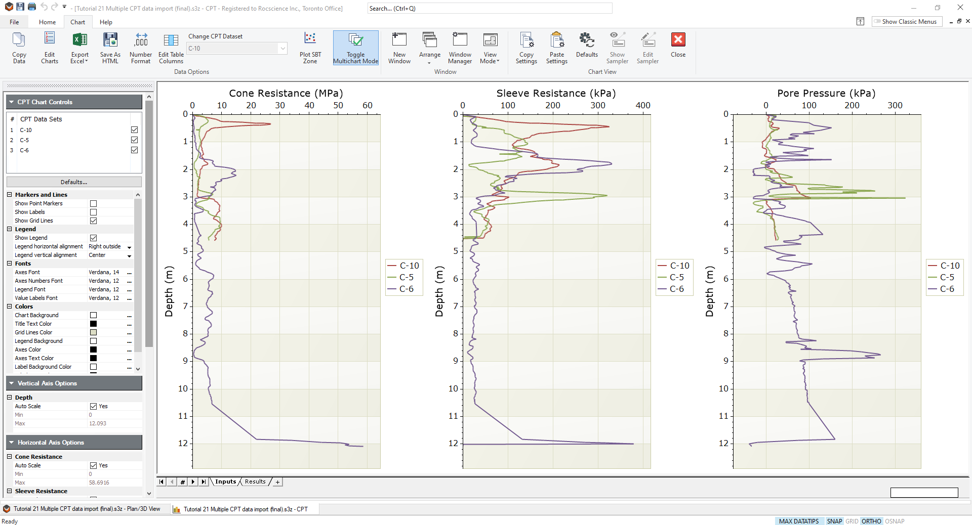
- Click the Toggle Multi-chart
 option right beside the drop-down menu to select different CPT data.
 - In the CPT Chart Controls check the boxes for the other two data sets.
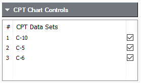
Then you will be able to see the results for all three data imported in one plot.
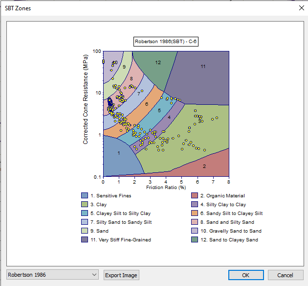
- You can also see the SBT (Soil Behavior Type) zone by selecting Plot SBT zone

Then you will be able to see the SBT zone for the CPT data as shown below. You can toggle different methods to see how this changes within the dialog.
5.0 Soil Profile
This feature also allows you to see the soil classification for delta size (m) of soil depth.
- Go back to the modeller, right-click and select CPT Soil Classification
 as shown below.
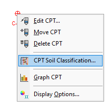
Then you will be able to see the soil classification with % for depth of soil defined as shown below for imported CPT data C-6: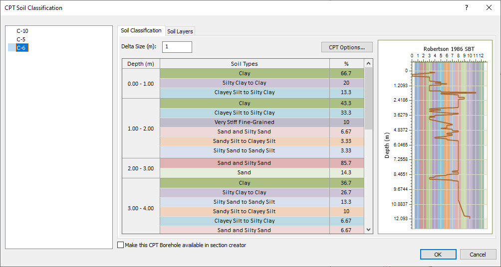
- Select the Soil Layers tab to see the soil profile with layer depth as overall layout of the soil layer column.
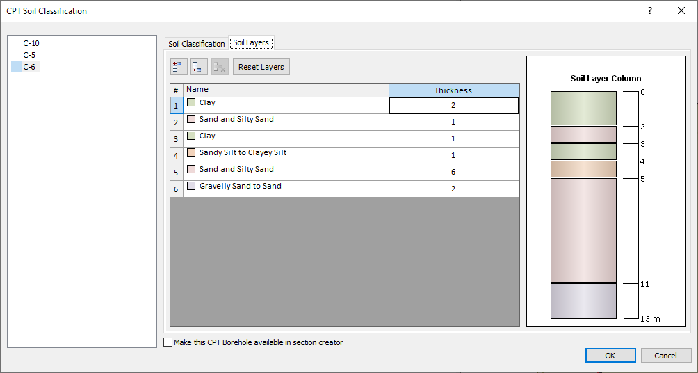
- Click OK to close the dialog.
6.0 Additional Exercise
The CPT Simulation feature can be used when you have more than two CPT points in the model. First, we will simulate points between the three CPTs we have imported in this tutorial.
6.1 CPT Simulation
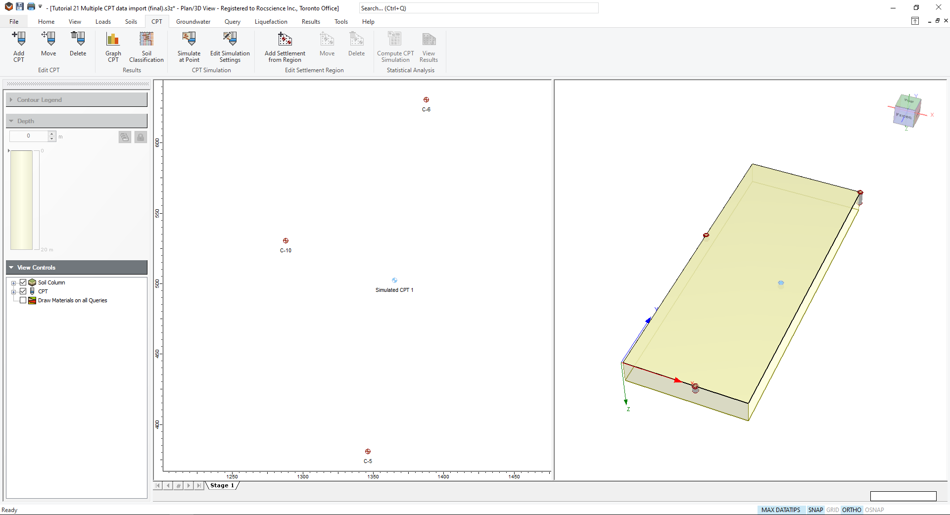
- Select CPT > Simulate at Point

The Simulate at Point dialog will open, where Parameters and Points settings can be defined.
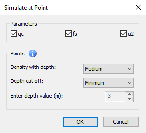
Parameters allow you to simulate the parameter of choice, and points allow you to define the density of your simulation for CPT points, and depth at which the points will be generated.
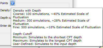
Hovering over the Info icon will allow you to see more details on the different options for Points. Keep in mind, your selection will affect computation time (Coarse = faster, Fine = slower).
- For the Density at Depth value, select Medium.
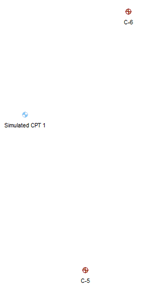
- Select anywhere between CPT points C-5 and C-6. After the simulation is completed, the symbol will indicate the simulated CPT is ready, by changing from grey to blue.
- Right click on Simulated CPT point and select Edit CPT.
- In the Edit CPT dialog, you will see the simulated CPT data points. Data cannot be modified here, however, you can select and copy the cells to other programs.
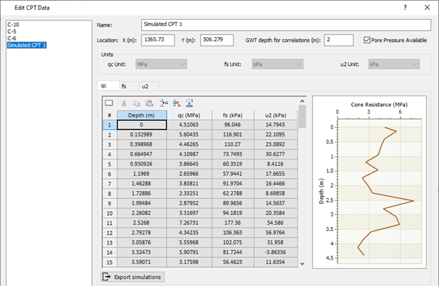 Note that the values here are an average of all the simulations. To see all simulated results, select Export Simulations.
 - If you place the CPT simulations near the CPT input and change Density with Depth to Fine, note that the simulated CPT is similar to the input CPT.

As shown in the graphs above, the simulated point is similar to the C-10 CPT points.
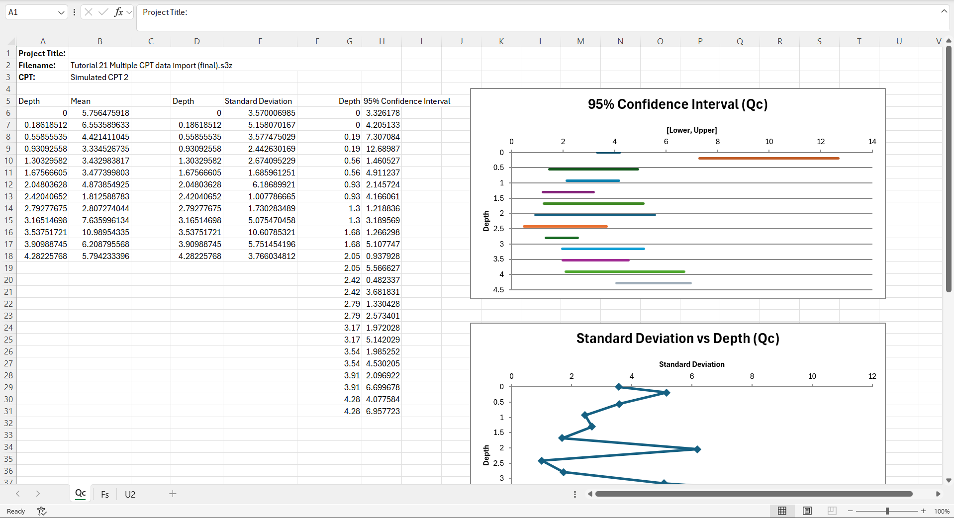
- To view the CPT simulation statistics, right-click on the simulated CPT and select Export Statistics to Excel. This will create an Excel file containing three worksheets, one for Qc, Fs, and U2. Within these sheets, you will find the 95% confidence interval, standard deviation, and mean values for the simulation
6.2 CPT Settlement
You can use the Add Settlement from Region option to simulate Schmertmann’s empirical settlement with simulated CPT points.
- Select CPT > Add Settlement from Region

- You will see the Add Settlement Region dialog, which allows you to define the foundation size, number of grid points, and density of the simulated parameters. Refer to the CPT Theory Manual for details on CPT settlement.
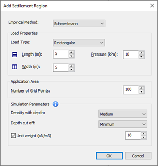
The Unit weight option allows you to assign constant unit weight along the depth of soil. Alternatively, you can allow the unit weight to be simulated at the cost of computation time. - Click OK. You will then be prompted to define each of the grid points within the region, using the dimensions provided in the Add Settlement Region dialog.
Enter the coordinates using your mouse or enter "t" in prompt line to use the coordinate table option.
x y 1280 300 1650 280 1700 400 1400 700 1200 650 1150 480 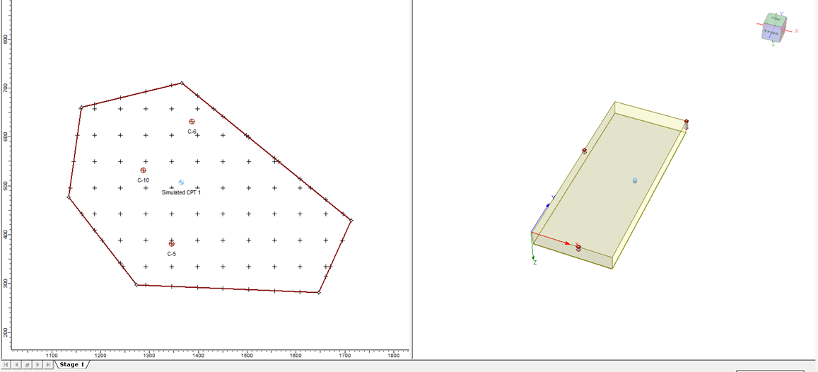
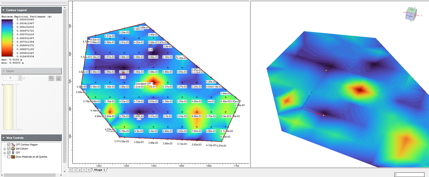
- Click Compute CPT Simulations
 . Depending on the your settings, you may be prompted with a warning message regarding a longer computation time.
Once the results are computed, the results window will open. Here, you can see the contour of the settlement. All the grid points are shown with the settlement results.
This concludes the additional exercise of the simulated CPT and CPT settlement feature.