9 - Empirical Methods

1.0 Introduction

This tutorial introduces empirical methods used calculating settlement such as Schmetimann, Peck, Thornburn and Hanson, and Schultze and Sherif method. It also shows the use of an info viewer to see the results.

Finished Product:

The finished product of this tutorial can be found in the Tutorial 09 empirical settlement methods.s3z file. All tutorial files installed with Settle3 can be accessed by selecting File > Recent Folders > Tutorials Folder from the Settle3 main menu.

2.0 Model

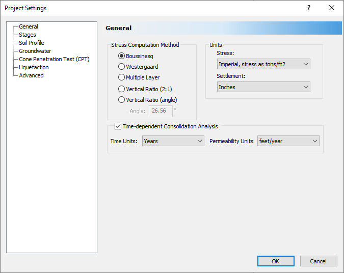
2.1 Project Settings

1. Select Home > Project Settings
2. Set the Stress Units = Imperial, stress as tons/ft2 and the Settlement Units = Inches. Select the Time-dependent Consolidation Analysis checkbox and set the Time Units = Years and Permeability Units = feet/year.
   
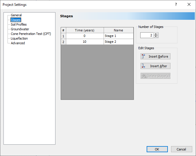
3. Click on the Stages tab. Click the Insert After button to add a new stage. Set the time to 10 years.
4. Select the Soil Profile tab. Select the 'Depth below Ground Surface' option.

5. Click OK to close the dialog.

3.0 Assign Water Level

1. Select Groundwater > Add Piezometric Line from the menu.
2. Set the Depth to 13 ft. and click OK.
3. In the Assign Piezometric Line to Soils dialog, click on Select All, then click OK.

4.0 Adding a Load

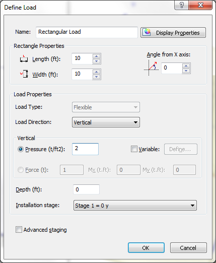
We will simulate the construction of a footing in Stage 1.

1. Select Loads >Rectangular Load
2. Set the Length and Width to 10 feet.
3. Set the Depth to 3 feet and the Pressure to 2 t/ft2 as shown.



4. Click OK.
   
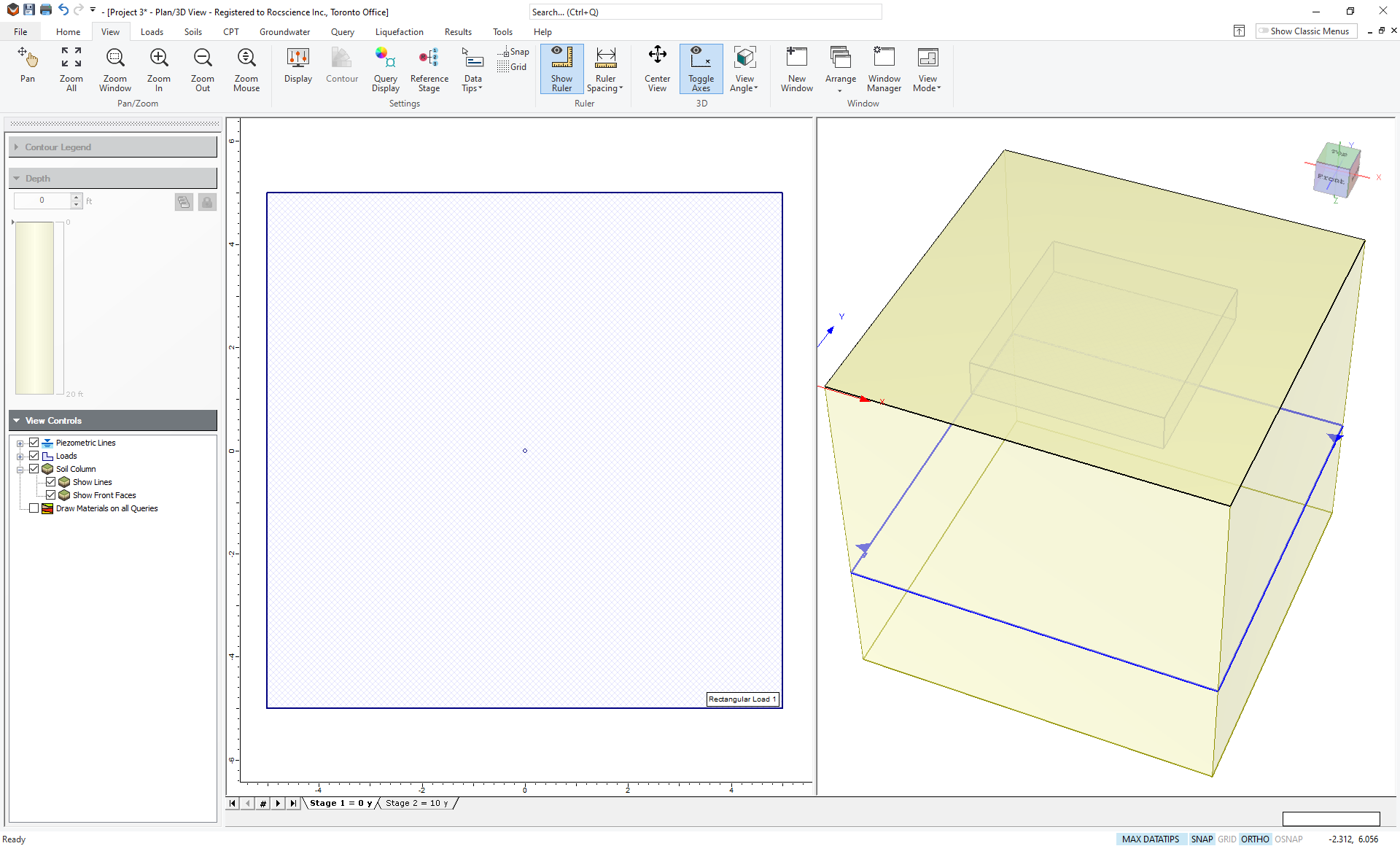
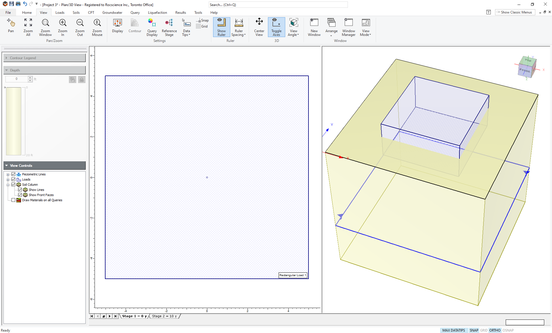
   You will now see a rectangle that needs to be placed somewhere on the Plan View. You can use the mouse to place the load, or alternatively, you can enter the coordinates in the prompt line at the bottom right of the screen.

5. Enter {0,0} and hit Enter to place the center of the load at the {0,0} coordinate in the Plan View.

You should now see the rectangular load in both the plan view (left) and the 3D view (right). You can zoom to the extent of boundaries in the Plan View by going to the View menu and selecting Zoom > Zoom All (or by using the toolbar button shown).

Your model should now look like this:

It looks a bit strange because the top of the footing is plotting below the surface since we applied the load at 3 feet depth. To manually change the appearance:

1. Right-click on the load in the plan view and select Display Properties.
2. Set the Custom height to 5 feet as shown:
   
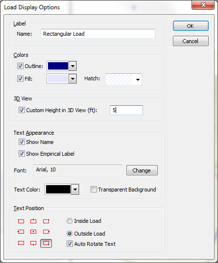
3. Click OK and the model should look like this:
   

5.0 Soil Properties

It is not really necessary to set up material properties and thicknesses when performing empirical analyses. You can specify different material configurations for each empirical method and for each load (if, for example, the soil is known to exhibit different properties at different locations). In this example, we only have one load so it will be easier to set up the soil layers and use them for each method.

For this tutorial, we will assume three layers of sand of increasing stiffness with depth.

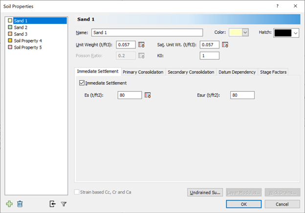
1. Select Soils > Define Soil Properties
2. Turn on Immediate Settlement and turn off Primary Consolidation settlement.

3. Set the Unit Weight and Saturated Unit Weight to 0.057 t/ft3.

4. Set Es and Esur to 80 t/ft2.

The dialog should now look like this:

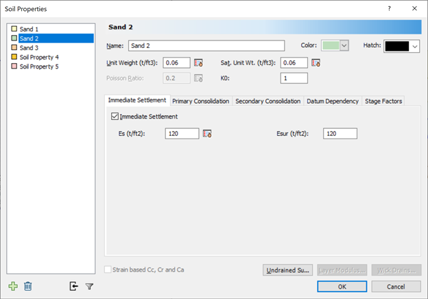
5. Click on the tab for Soil Property 2. Set the properties as shown:
   • Name = Sand 2
   • Unit Weight = 0.06
   • Sat. Unit Wt. = 0.06
   • Turn on Immediate Settlement and turn off Primary Consolidation settlement
   • Es = 120
   • Esur = 120

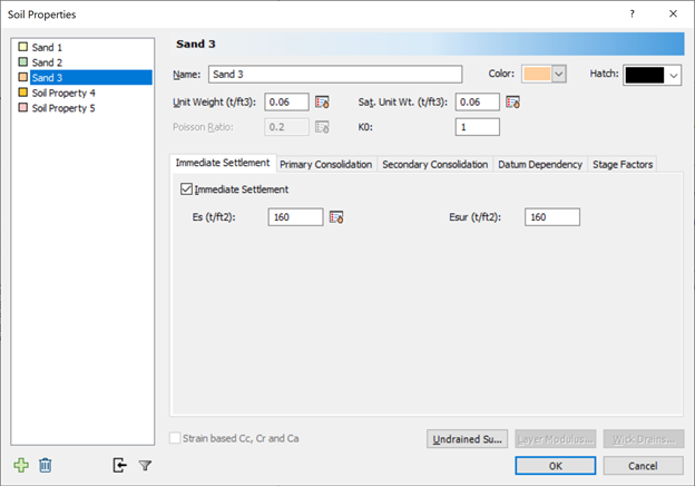
6. Now set the properties for Soil Property 3.
   • Name = Sand 3
   • Unit Weight = 0.06
   • Sat. Unit Wt. = 0.06
   • Turn on Immediate Settlement and turn off Primary Consolidation settlement
   • Es = 160
   • Esur = 160

7. Click OK.

6.0 Soil Layers

1. Select Soils > Layers
2. Change the thickness of the first soil layer (Sand 1) to 5.
3. Click the button for Insert Layer Below twice to add two layers.
4. Set the thickness of the second layer (Sand 2) to 8 and the bottom layer (Sand 3) to 10 as shown.



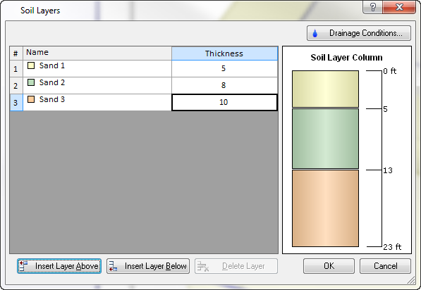
5. Click on the Drainage Conditions button, and make sure that the Drained Ground Surface checkbox is selected in the Soil Drainage Conditions dialog.
6. Click OK to close the dialogs.

7.0 Empirical Settlement Calculation

We will use the material properties and layer thicknesses as a basis for the empirical settlement calculations. However, each method may require a different type of input, for example, blow counts from an SPT test rather than Young's modulus. We will examine the input for each method in turn.

7.1 Limitations of empirical methods

Because the empirical methods are based on observed settlement results from actual field studies, the methods do not capture every possible loading scenario. The empirical methods have certain limitations as follows:

• Calculations can only be performed for circular and rectangular loads. There are no solutions for irregularly shaped loads or embankments.
• The material is assumed to be some type of non-cohesive sand and the settlement is assumed to occur immediately (although the Schmertmann method does account for creep).
• Loads are assumed to be rigid, so the settlement is the same everywhere over the load area.

We will go through the different calculation methods now.

7.2 Schmertmann

The Schmertmann method calculates settlement from layer stiffness data or cone tip bearing resistances, q_c obtained from a Cone Penetration Test (CPT). The method proposes a simplified triangular strain distribution and calculates the settlement accordingly. A time factor can also be included to account for time-dependent (creep) effects.

1. Select Loads > Empirical Methods > Schmertmann. You are now prompted to choose a load.
2. Click on the square load and hit Enter. The Schmertmann dialog will now appear.
3. Select the Calculate checkbox at the top of the dialog. You can now enter material properties and choose various analysis options.
4. Click the Copy from Soil Layers button. The layers, thicknesses and unit weights that we previously entered in the Soil Layers dialog, will be copied to the Schmertmann dialog.

By default, the Schmertmann method displays the CPT-bearing resistance q_c for each layer. This is estimated by taking half of the entered values for Young's modulus (E_s). This estimate may not be accurate depending on the soil type etc., so you can change the values in this dialog. However, for this analysis, we will use the estimated values. Traditionally, when doing a Schmertmann analysis by hand, the practitioner must set up many layers to get an accurate strain profile with depth. Settle3 sets up many layers automatically (if the Auto Subdivisions option is chosen). Therefore we only need to set up separate layers if they have different material properties.

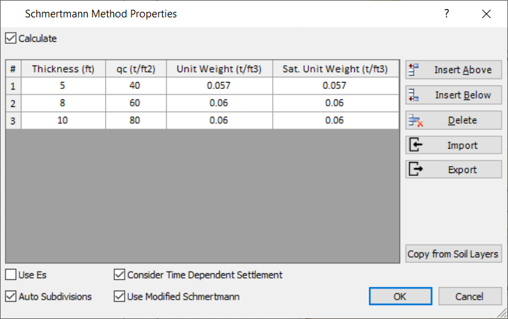
5. Be sure to check the box to Consider time-dependent settlement and the box to Use modified Schmertmann (this is a modification of the original Schmertmann method that is often regarded to give more accurate results – see the Theory Manual for more details).
6. Click OK and you will now see the calculated settlement displayed at the bottom right corner of the load in the Plan View, as shown.

7.3 Peck, Hanson and Thornburn

The method of Peck, Hanson and Thornburn (1974) uses the results of a Standard Penetration Test (SPT) to obtain settlement. The water table and overburden pressure at the location of the SPT are taken into account. Settlement results are obtained from matching the problem geometry and corrected SPT results to empirical curves.

1. Select Loads > Empirical Methods > Peck, Hanson, Thornburn.
2. Click on the square load and hit Enter.
3. In the resulting dialog, check the box for Calculate. You are now asked to enter some material parameters. As with the Schmertmann method, you can define multiple layers. Click the Copy from Soil Layers button. You will now see the three layers with their thicknesses and unit weights.

The blow count, N₆₀ represents the blows per foot from an SPT test, corrected to account for the efficiency of the hammer. See the Theory Manual for more information. Settle3 does not know how to convert from Young's modulus to blow counts, since the relationship is highly dependent on the material type. Peck et al. suggest the following relationship:

Assuming we have medium sands, we can convert the Schmertman q_c values to N₆₀ by dividing by 4. This yields values for N₆₀ as shown:

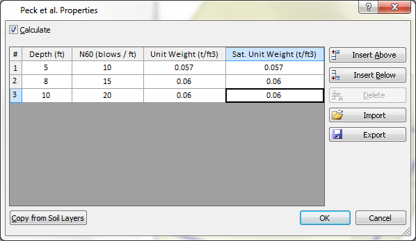
4. Fill in these values for N₆₀ (as shown above).
• Layer 1 = 10
• Layer 2 = 15
• Layer 3 = 20
5. Click OK to close the dialog.

You will now see the results of the Peck, Hanson and Thornburn analysis on your plot, as well as the Schmertmann results.

7.4 Schultze and Sherif

As with the Peck, Hanson and Thornburn method, the Schultze and Sherif method also uses the blow counts to calculate the settlement. No corrections are made for overburden depth so unit weights are not required. We will now demonstrate an alternative method of applying an empirical analysis, using a right-click shortcut.

1. Right-click on the square load.
2. From the pop-up menu, select Loads > Empirical Methods > Schultze + Sherif.
3. Check the Calculate checkbox.
4. Select the Copy from Soil Layers button.
5. Enter the same N₆₀ values you used for the Peck et al. method as shown.
   
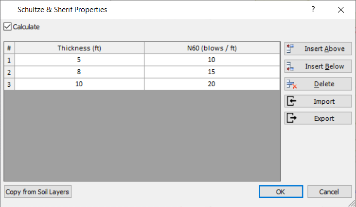
6. Click OK to close the dialog and see the results.
   

8.0 Result comparison and analysis

Select Results > Report Generator. Here you can see all of the information relating to your model. Scroll down until you see the summary of Empirical Results.

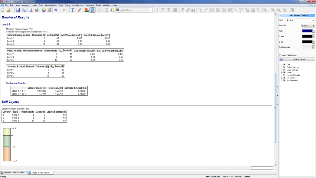
Here you can easily compare the settlements calculated using the different methods.

The Peck, Hanson and Thornburn method is often considered to be conservative and the calculated settlement is often multiplied by two-thirds to get a more realistic answer (Peck and Bazarra, 1969). This would yield a settlement of 0.69 inches – about halfway between the values calculated with the Schultze and Sherif method (0.39) and the Schmertmann method (0.96 inches). These discrepancies highlight how the empirical methods can give quite different results for the same problem, since different assumptions are made with each method.

This concludes the tutorial; you may now exit the Settle3 program.

9.0 Additional Exercises

1. Assume that the material is a coarse sand, in which case N₆₀ = q_c / 6. You should now see settlements for the Peck et al. method and the Schultze and Sherif method that are closer to those calculated using the Schmertmann method (if you apply the two-thirds correction for the Peck et al. method).
2. Change the load properties and set the load type to rigid instead of flexible. You will need to turn off the time-dependent analysis before you can do this. Put a query point in the middle of the load to compute the settlement. Compare this settlement to the values calculated using the empirical methods.

The value of 1.03 inches is the same for both stages since there is no time-dependent component to this analysis. The settlement compares well with that calculated using the Schmertmann method.

10.0 References

Peck, R. B. and Bazarra, A. 1969. "Discussion of Settlement of Spread Footings on Sand," by D’Appolonia, et. al, Journal of the Soil Mechanics and Foundations Division, 95, 905-909.

Peck, R.B., Hanson, W.E. and Thornburn, T.H., 1974. Foundation Engineering, 2^nd edition, John Wiley and Sons, Inc.