14a - Liquefaction analysis using CPT data

1.0 Introduction

In Settle3, liquefaction analysis can be performed using SPT, CPT, and VST data. This tutorial provides an introduction to the liquefaction analysis using CPT data in Settle 3. Before proceeding with the tutorial, make sure you’ve gone through Tutorial 14 - CPT analysis in Settle3 so you’re familiar with the product’s basic functions and features related to CPT analysis.

Topics Covered in this Tutorial:

• CPT data interpretation
• Liquefaction analysis using CPT data

Finished file:

The finished file of this tutorial can be found in the Tutorial 14a Liquefaction analysis using CPT data.s3z file. All tutorial files installed with Settle3 can be accessed by selecting File > Recent Folders > Tutorials Folder from the Settle3 main menu.

2.0 Model

2.1 Project Settings

1. Select Home > Project Settings (CTRL + J) to open the Project Settings dialog.
2. In the General tab, make sure the Stress Units are set as Metric, stress as kPa and the Settlement Units are set as Millimeters.
3. Go to the Cone Penetration Test (CPT) tab and check the CPT Analysis checkbox to turn the CPT analysis option on.
   
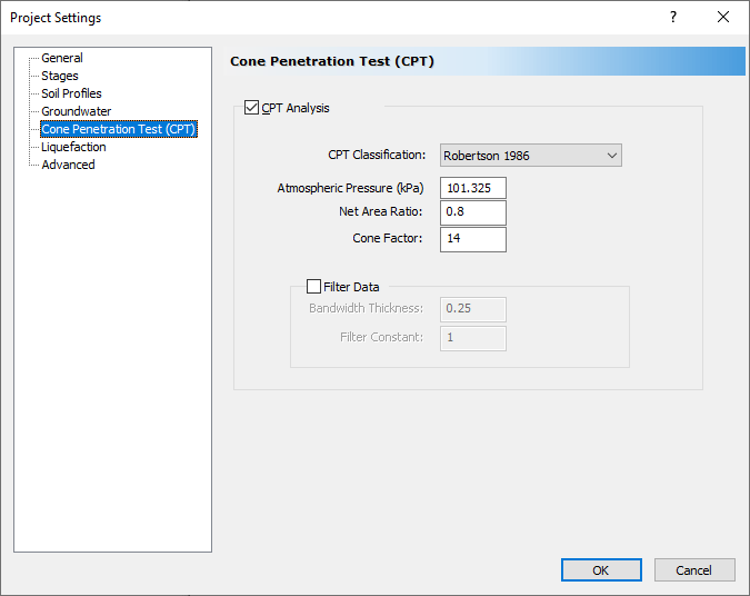
4. Go to the Groundwater tab and check the Groundwater Analysis checkbox to turn the groundwater analysis option on.
5. Click OK to close the dialog and save your changes.
You may be warned that the unit system has changed. If this is the case, select Yes to reset the unit-dependent values.

3.0 Enter CPT Data

1. Select CPT > Add CPT icon in the toolbar to open the CPT Input dialog.
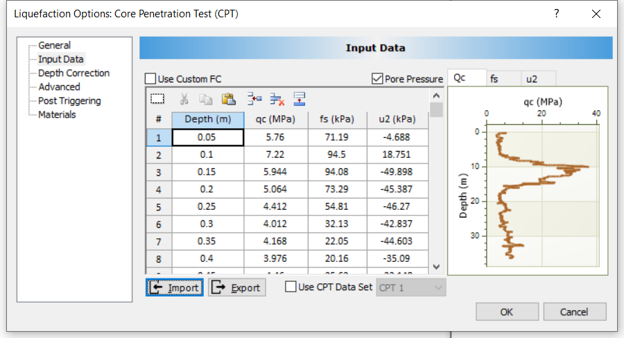
2. Click Import button and import the file CPT_Input_liquefaction.txt.
3. The Import Data dialog will appear. Make sure Auto Detect Data is checked and data delimiter should be space. You should see the following:



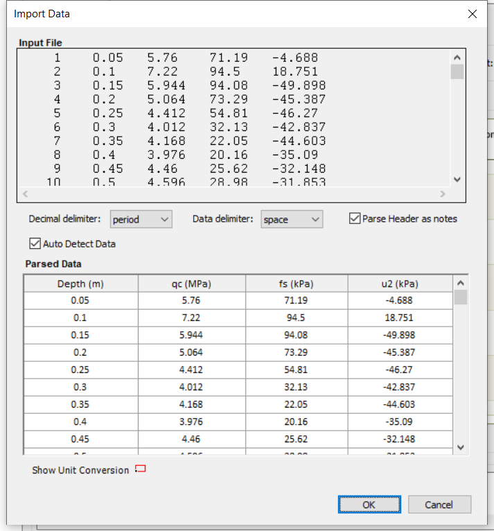
4. Click OK to return to the previous dialog.
5. Leave the GWT depth for correlations equal to 2 m and the Location of the CPT point to 0,0.



6. Click OK to close the dialog.

3.1 Soil Profile

1. Right-click on the CPT point and select CPT Soil Classification . You should see the soil types defined for each increment of depth with a delta size (m) of 1.
   
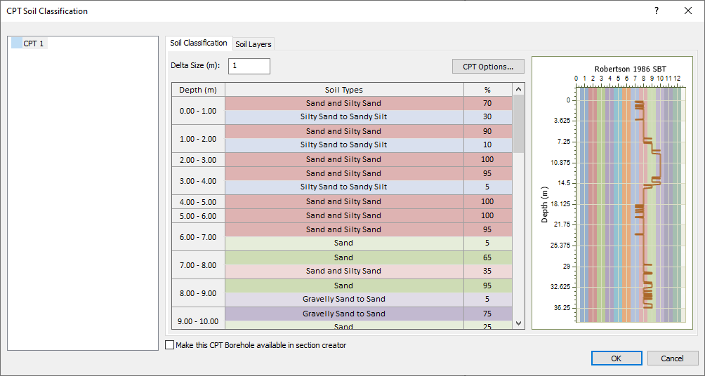
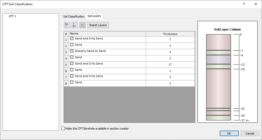
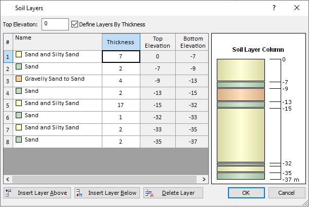
2. Select the Soil Layers tab. The consecutive soil layers are automatically merged to the soil profile shown below:
   
   
3. Click OK.
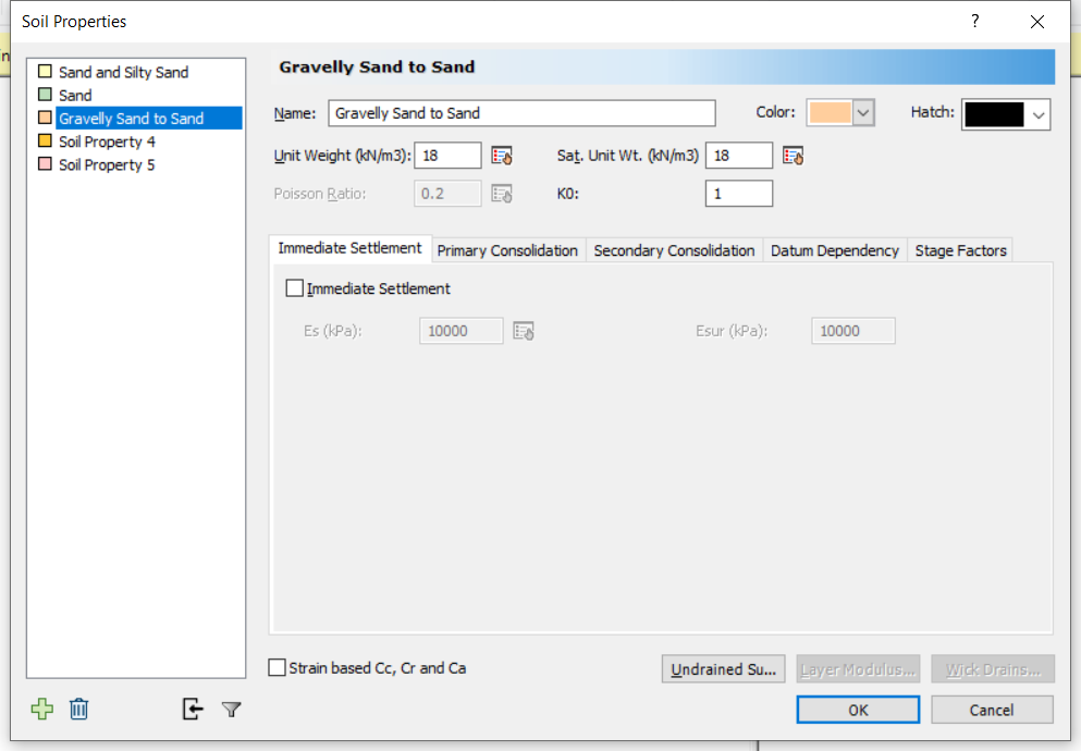
4. Select Soils > Define Soil Properties
5. Change the name of the following soil properties:
• Soil Property 1: Sand and Silty Sand
• Soil Property 2: Sand
• Soil Property 3: Gravelly Sand to Sand
We have deleted soil property 4 and Soil property 5 for visual purposes as they're not used, but there's no need to delete these layers as they won't be used.



6. Click OK to close the dialog.
7. Select Soils > Layers
8. Click the Insert Layer Below button to create 7 new layers (8 layers in total).
9. Assign the following soil layers and enter the following thicknesses as shown:
• 1. Sand and Silty Sand = 7
• 2. Sand = 2
• 3. Gravelly Sand to Sand = 4
• 4. Sand = 2
• 5. Sand and Silty Sand = 17
• 6. Sand = 1
• 7. Sand and Silty Sand = 2
• 8. Sand = 2



10. Click OK.
    

3.2 Groundwater table

After CPT data is located in the modeller, now we will assign a water table to the soil profile.

1. Select Groundwater > Add Piezometric line.
2. Add Piezometric line with Depth(m) of 0 m. Then, Assign to all materials and select OK.
   
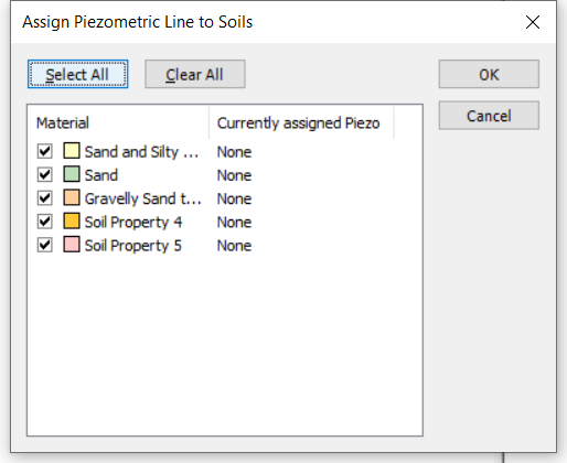
3. Select OK and you will see that piezometric line is applied to the soil profile.
   

4.0 Liquefaction Analysis

After CPT data is imported, we will be using this data for liquefaction analysis. Firstly, we need to enable the liquefaction analysis option in Settle3.

4.1 Project Settings

1. Go to Project settings and select the Liquefaction tab.
2. Turn on the Liquefaction analysis and select CPT data as shown below:
   
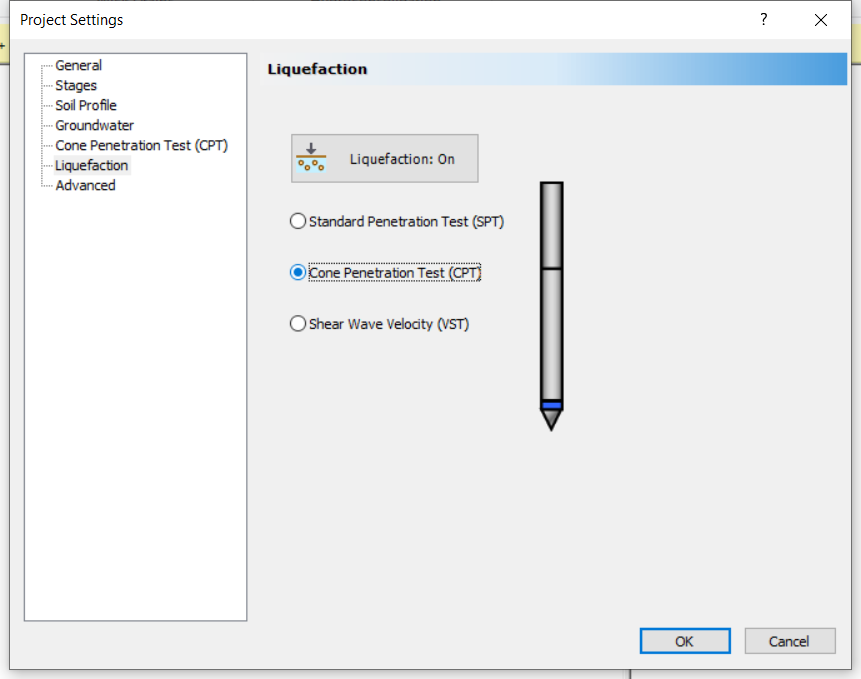
3. Select OK.
   

4.2 Liquefaction options

1. Select Liquefaction > Liquefaction Options
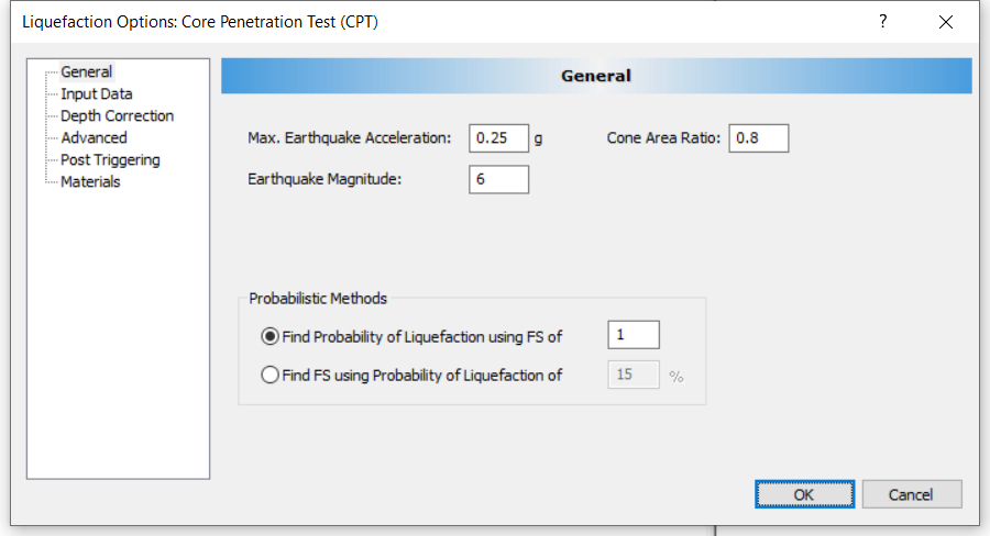
2. Under the General tab, change the value of the following parameters to the following:
• Max. Earthquake Acceleration: 0.25 g
• Earthquake Magnitude: 6
• Cone Area Ratio: 0.8
• Keep probabilistic methods: Use FS of 1.



3. Under input data, select Import button, and import CPT data_liquefaction.txt. The import data dialog will appear.
4. Make sure Auto Detect Data is checked and data delimiter should be space.
5. Click OK to return to the previous dialog
6. Uncheck 'Use Custom FC Threshold'.
   
7. Under the Advanced option, set Magnitude Scaling Factor (MSF) to Idriss (NCEER) and Stress Reduction Factor (Rd) to NCEER (1997).
   
   
8. Under the Post triggering method, select 'Calculate Dry Sand Settlement' and keep calculate settlement for FS < 1.
   
9. Select the Materials tab and select each material property and change the values for the parameters as the following:
• Material: Sand.
• Fines Content: 2 %
• D50: 3 mm
• Check Prone to Liquefaction
• Material: Sand and silty sand.
• Fines Content: 3 %
• D50: 2 mm
• Check Prone to Liquefaction
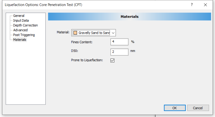
• Material: Gravelly Sand to Sand.
• Fines Content: 4 %
• D50: 2 mm
• Check Prone to Liquefaction



10. Select OK to close the dialog.

4.3 Liquefaction Analysis Options

Now we will decide which methods we want to use to analyze the liquefaction.

1. Select Liquefaction > Analysis options.
   
   In this option, users can choose different methods for triggering method, settlement, dry settlement, and lateral displacement options.
   
2. In this tutorial, we will use Idriss and Boulanger (2014) and Moss et al. (2006) Probabilistic for Triggering - CPT.
3. Check the Settlement option for Yoshimine et al. (2006), and select both options available for Lateral Displacement. The dialogue should be as shown below:
   
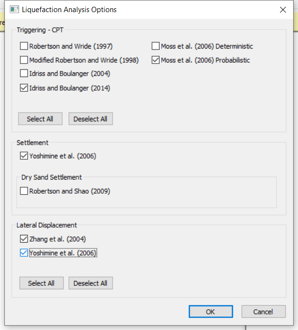
4. Click OK.
   

4.4 Liquefaction analysis results

In order to see the liquefaction analysis results, you have to create a query point on the soil model to analyze the liquefaction.

1. Create query point by selecting Query > Add Point
2. Create query point close to CPT data (ex. 0.5 meter away from CPT data as shown. Note that color scheme of materials may vary with the image below).
   
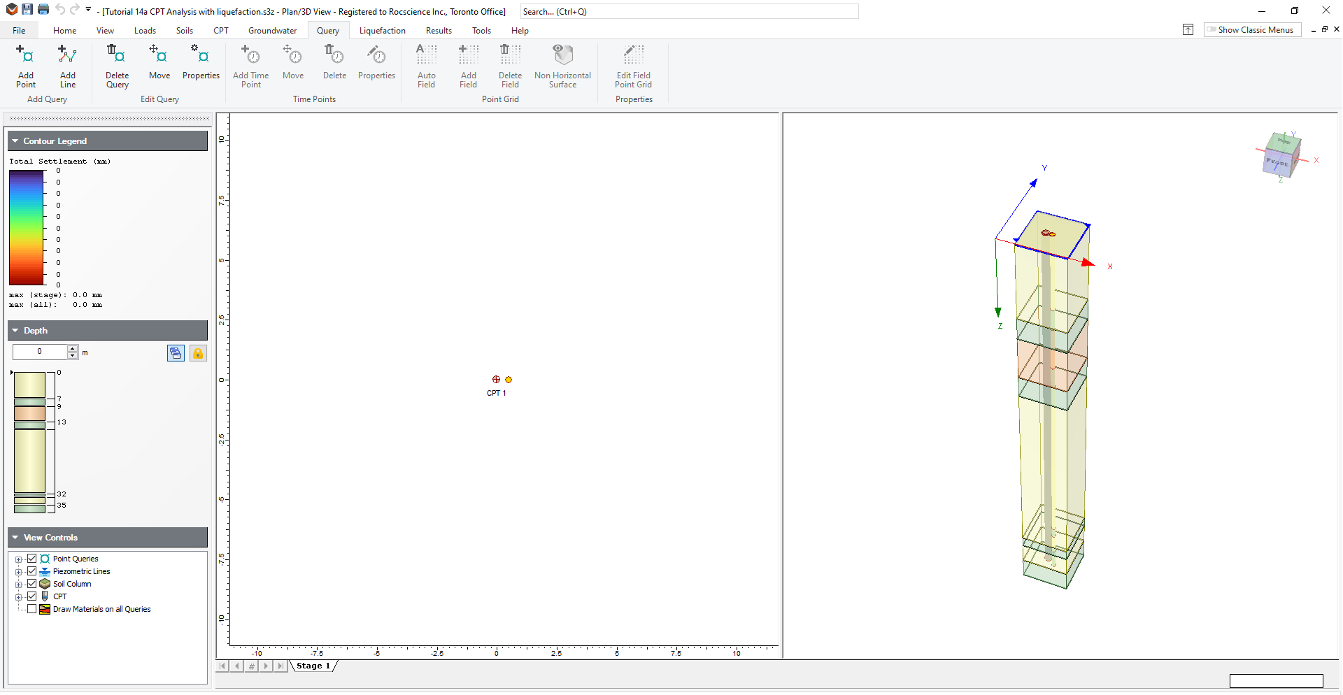
3. Right-click on the query point and you will see that 'Graph liquefaction' is available.
   
If you do not see this option enabled, check step 3.2 of this tutorial where the soil profile has a groundwater table assigned.
4. In the Plot Liquefaction dialog, click OK. You will see the following results for Data.
   
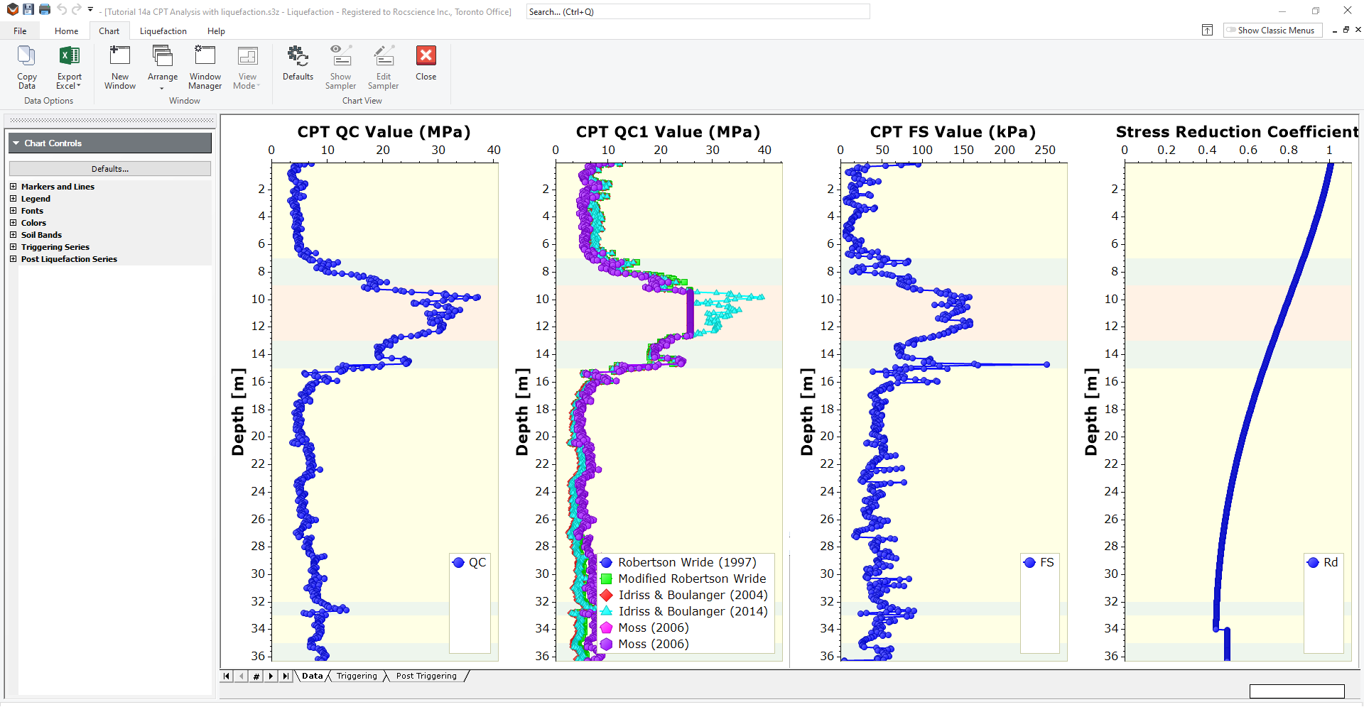
   You will notice that the region of Gravelly sand to sand region has a high QC value and QC1 value.
   
   
5. Now select the Triggering tab and you will see the results as shown below:

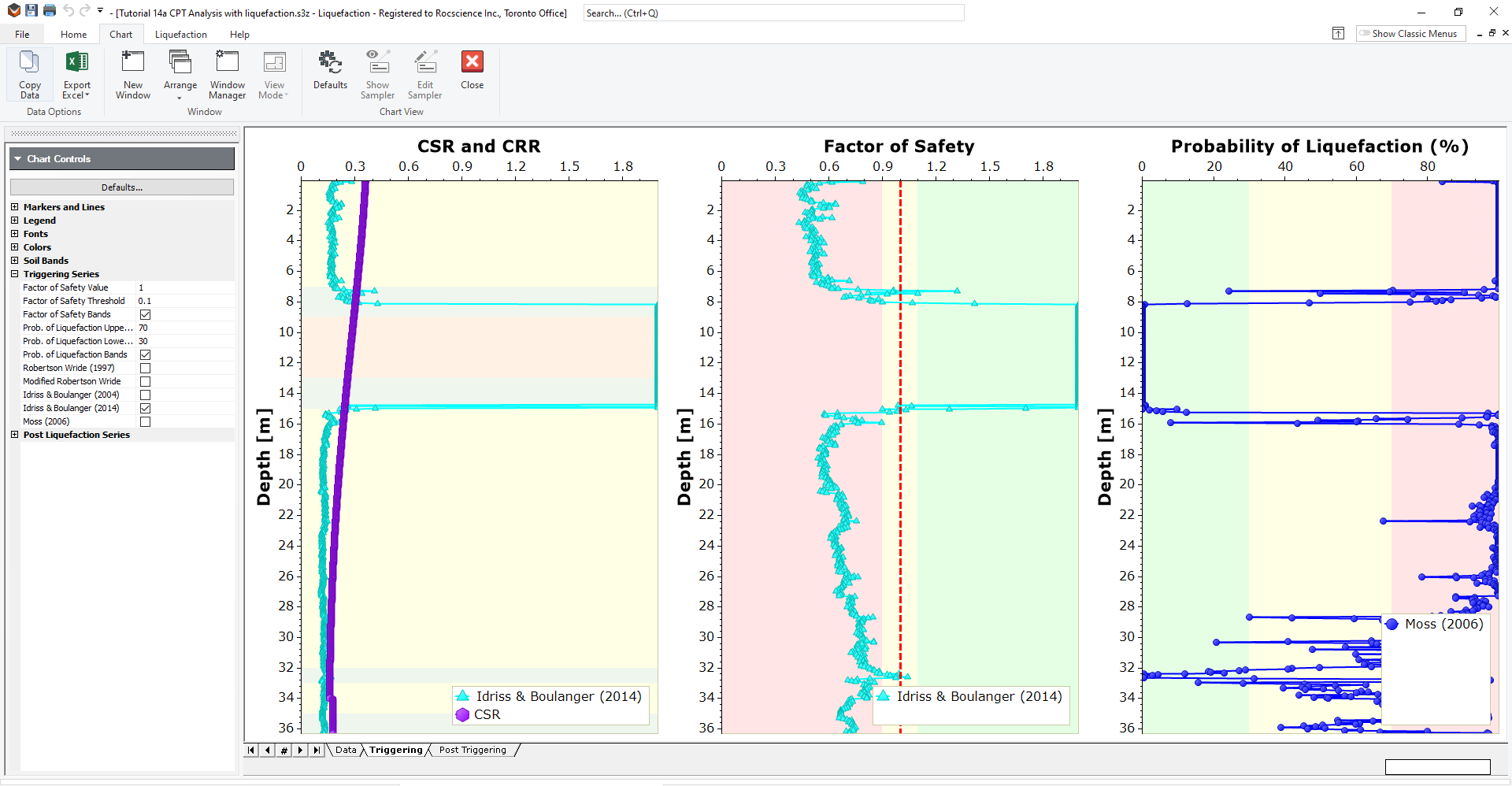
If you look at the CSR and CRR value, the Idriss method shows a high jump in the plot. In the factor of safety chart, you will see that the region of Gravelly sand to sand layer has very low susceptibility to liquefaction with a factor of safety above 1 while the other layers are susceptible to liquefaction.

This can be observed closely in the probability of liquefaction (%) chart.

Now we will look at the Post Triggering tab.

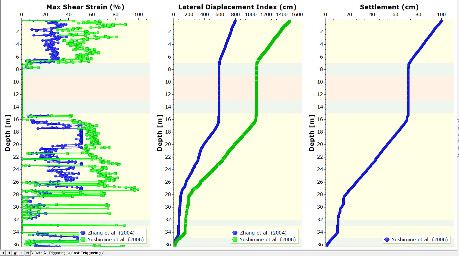
Two methods are used for the post triggering method (Zhang et al, and Yoshimine et al). You will see that at the region of low probability of liquefaction, there is less lateral displacement / max shear strain. lateral displacement and settlement is significant at the layers that are susceptible to liquefaction which is observed from the triggering tab.

Therefore, you can utilize the data, triggering, and post triggering tabs to analyze liquefaction and the lateral or settlement due to liquefaction.

This concludes liquefaction analysis with CPT data.