15 - Capacity Ratio of Reinforced Concrete Pile

1.0 Introduction

In this tutorial, a reinforced concrete pile is analyzed under axial load and biaxial bending conditions (combined section loading). The tutorial aims to define the needed steps to determine the structural adequacy of the section of a bored pile through the capacity ratio calculations.

The capacity ratio is defined in RSPile as demand ultimate moment/factored moment capacity at a specific ultimate load.

1.1 Model Description

For this tutorial, we will being using a pile that is 600mm in diameter and 15m long. The section of the pile is made of reinforced concrete with concrete cylinder strength of 32MPa, and 8 no. BS4449 25mm bars with a yield strength of 500MPa and a modulus of elasticity of 200GPa. The cover to the edge of the bars is 85mm. The section remains unchanged through the length of the pile.

The soil is chosen as elastic material having a modulus of 30MPa/m in the lateral direction and 10MPa/m in the vertical direction except for the tip where 100MPa/m is used.

The pile head is subject to a shear force of 250kN in each direction (x and y) and a couple of 250kN.m on each axis. An axial force of 2500kN downward is also applied at the top of the pile head.

Finished Product:

The finished product of this tutorial can be found in the Tutorial 15 - Capacity ratio of Reinforced Concrete Pile.rspile2 data file. All tutorial files installed with RSPile can be accessed by selecting File > Recent Folders > Tutorials Folder from the RSPile main menu.

2.0 Model

Using the information provided in the description above (on the pile, soil and loading given), we can begin to construct the RSPile model. Start by launching the RSPile program.

2.1 Project Settings

1. Select Home > Project Settings
2. In the General tab, set the Units as Metric and the Program Mode Selection as Pile Analysis.
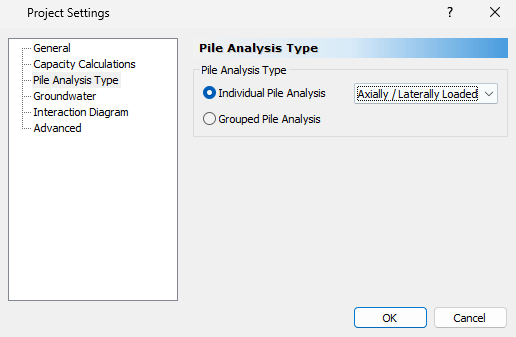
3. Select the Pile Analysis Type tab. The set the Pile Analysis Type as Individual Pile Analysis > Axially/ Laterally Loaded.
   
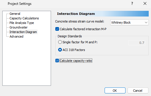
4. Select the Interaction Diagrams tab. For the Concrete stress strain curve model select Whitney Block.
5. Tick the box for Calculate factored interaction M-P. For Design Standards select ACI 318 Factors. Then tick the box for Calculate capacity ratio.
   
6. Select the Advanced tab. Increase the number of Reinforced Concrete Slices to 200.
This will help to get a smooth and continuous interaction diagram. The smaller the section, the higher the number of slices you need to get enough accuracy at the angle divisions for load direction and angle for neutral axis orientation. It seems that 200 will be good in most practical cases.
7. For Pile Discretization select Custom and then change the number of Pile Segments to 50 (so that we don’t have to calculate for a higher number of elements).
   
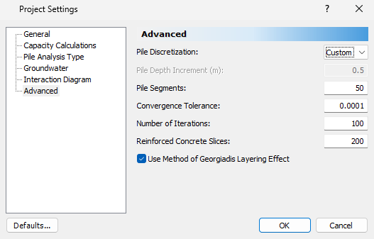
8. Click OK to close the Project Settings dialog.

2.2 Soil Properties

1. Select Soils > Define Soil Properties to open the Define Soil Properties dialog.
2. Select Soil Property 1 and change the Name to Elastic Soil.
3. Enter the following:
• Unit Weight (kN/m3) = 20
• Axial
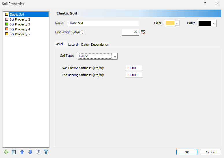
• Soil Type = Elastic
• Skin Friction Stiffness (kPa/m) = 10 000
• End Bearing Stiffness (kPa/m) = 100 000



• Lateral
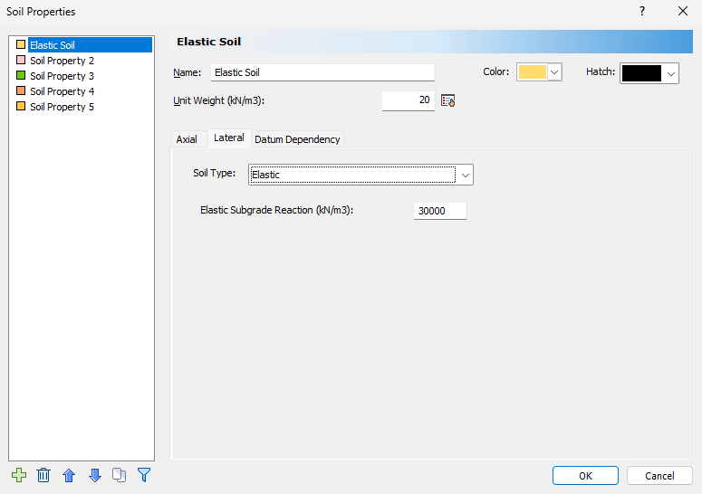
• Soil Type = Elastic
• Elastic Subgrade Reaction (kN/m3) = 30 000



4. Click OK.

2.3 Pile Sections

1. Select Piles > Pile Sections to open the Pile Sections dialog.
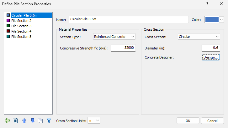
2. Use the Delete icon on the bottom left to delete the extra sections and keep only one. Change the Name to Circular Pile 0.6m. and fill the data boxes as shown below.
3. Enter the following:
• Section type = Reinforced Concrete
• Compressive Strength f'c (kpa) = 32 000
• Cross Section = Circular
• Diameter (m) = 0.6



4. Click the Design button to launch the Concrete Designer dialog.
5. In the Reinforcement tab, click the Add button to add a new reinforcement pattern.
6. Enter the following:
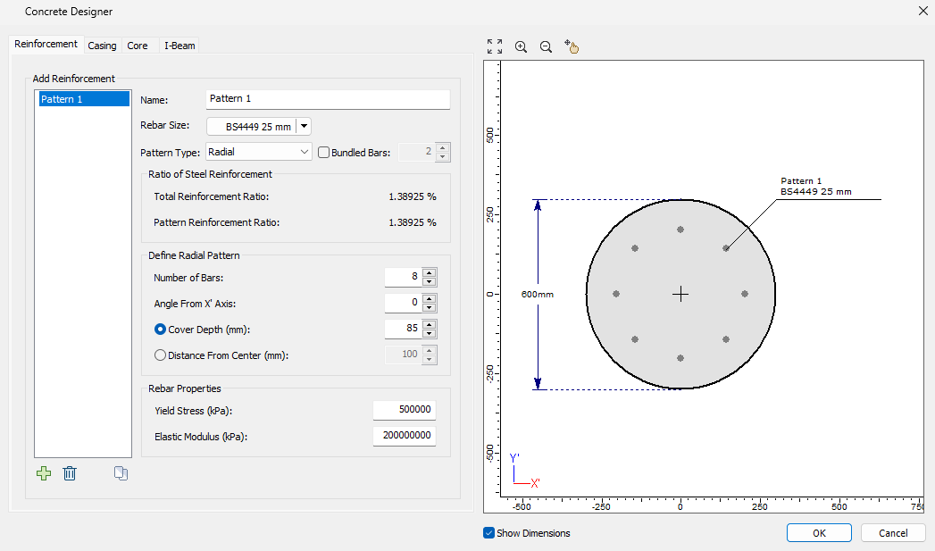
• Rebar size = Europe > BS4449 25mm
• Pattern type = Radial
• Number of Bars = 8
• Angle from X' axis = 0
• Cover Depth (mm) = 85
• Yield Stress (kPa) = 500 000
• Elastic Modulus (kPa) = 200 000 000



7. Click OK twice to close both the dialogs.

2.4 Pile Types

1. Select Piles > Pile Types in the menu to open the Pile Types dialog.
2. Select Pile Type 1 and change the name to Circular 0.6m Type.
3. Leave the Length as the default 15 m.
   
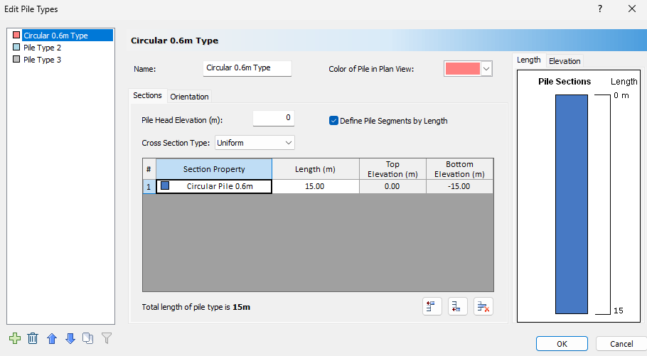
4. Click OK to close the dialog.

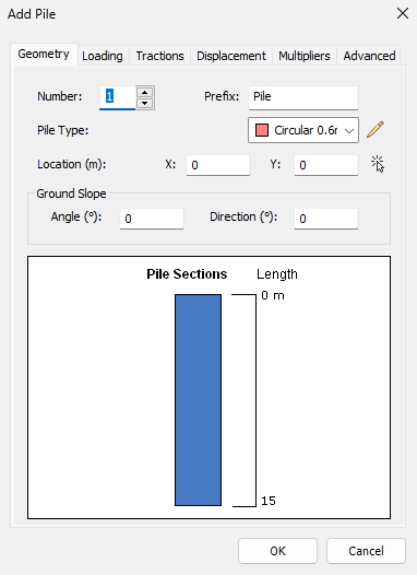
2.5 Add Pile

1. Select Piles > Single Pile in the menu to open the Add Pile dialog.
2. The Pile type we defined should be selected. We will use the default Location (m) = (0,0) for the pile.
   
3. Select the Loading tab. Click on the Add button to add a Load Property.
4. The Loading Property should be Static and the Loading Direction = General.
5. Click the Add button at the bottom left of the dialog to add the following Loading Conditions.

Type	Value	Depth (m)
Shear X (kN)	150	0
Shear Y (kN)	150	0
Moment X (kNm)	-250	0
Moment Y (kNm)	250	0
Force Z (kN)	-2500	0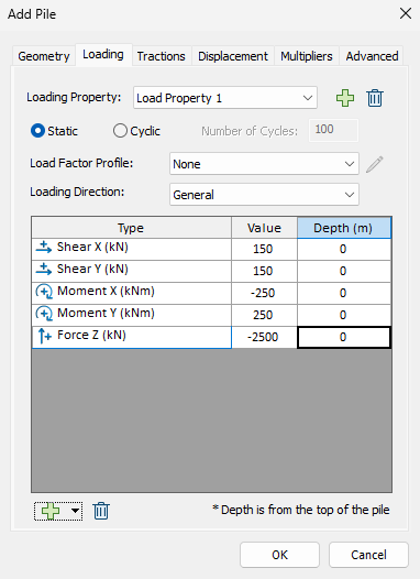



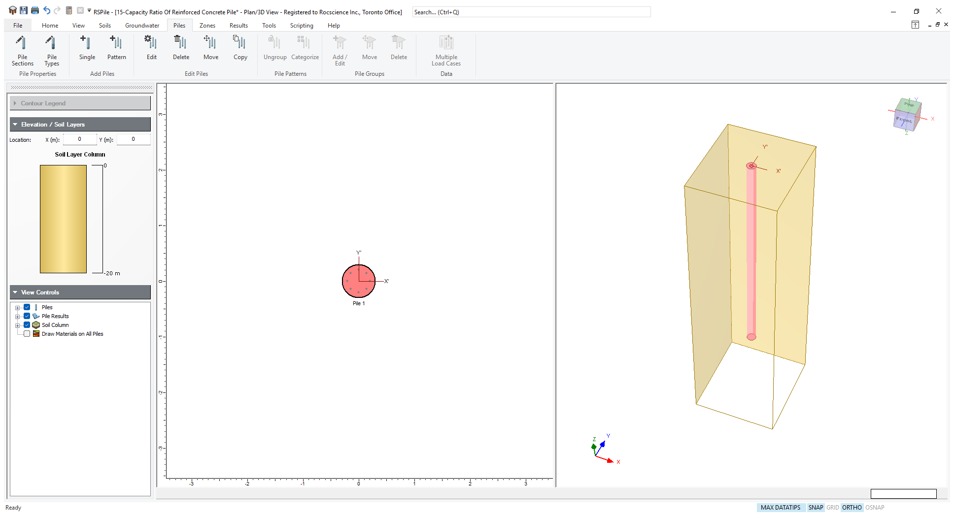
6. Click OK to place the pile.

The pile will appear in the main layout ready to be analyzed.

3.0 Pile Analysis

1. Select Results > Compute to execute your analysis.

This will take a couple of seconds. This is because it is getting enough points to define the interaction surface.

To see the results of the pile analysis:

1. Select Results > Graph Pile and use your mouse to select the pile, or right-click on the pile and select Graph Pile.
   
   You will get the results plotted and tabulated on the screen as shown below.
   
2. Select Chart > Edit Table Columns . In this dialog you can choose whatever data you want to see from the results. Select Beam Capacity Ratio and use the arrow button to add Beam Capacity Ratio to the Columns on display. Click OK.
   
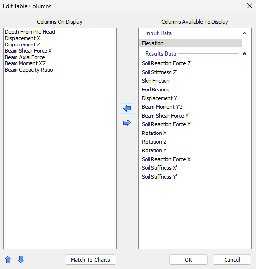
3. You can do the same for the graphs by selecting Chart > Edit Charts . To quickly match the graphs to the table columns, click Match to Table. Click OK to close the dialog.

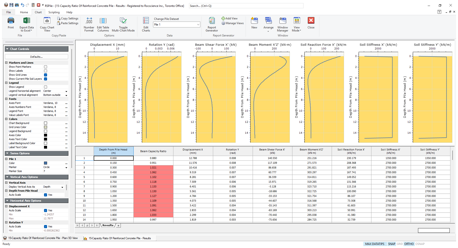
You may see some of the cells under capacity ratio red filled. These are the levels where the capacity ratio exceeds unity signaling inadequacy for the demand/capacity ratio.

The designer should change their section to have more strength at these levels.

4.0 Interaction Diagrams

To view the interaction diagrams for the pile section:

1. Go back to the model view by selecting the tab at the bottom of the screen.
2. Select Results > View Interaction Diagram
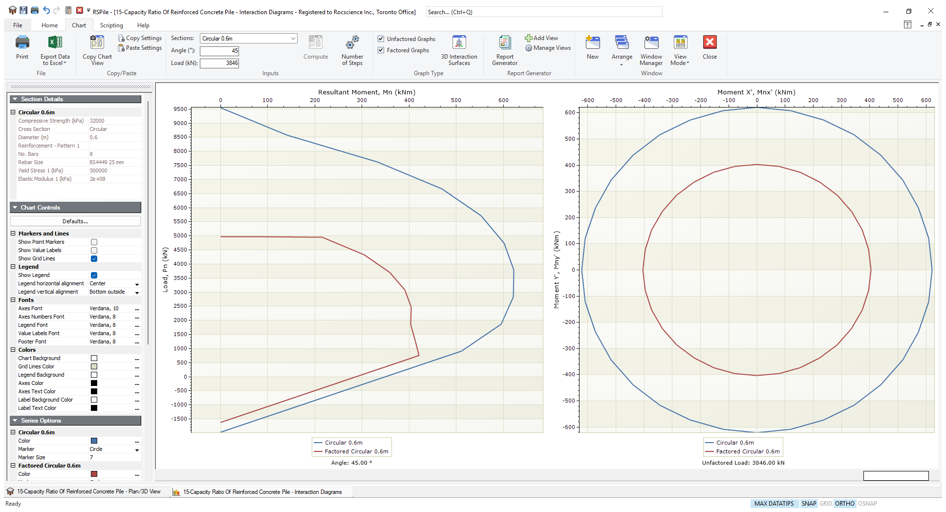
3. In the Chart tab, use the Sections drop down to select the Circular Pile 0.6m section.
4. Under Inputs enter a P-M Curve with an Angle of 45 degrees. For the Mx'-My' Curve enter Axial Load = 3846 kN
   
5. Click Compute . The Interaction Diagrams view will appear.
6. Under Graph Type, tick the box for Factored graphs. You should now see both the factored and unfactored interaction diagrams.
   
   
7. To change the angle or the load, you can do so easily by updating the Angle and/or Load fields and clicking Compute again.

It should be noted that the load chosen is unfactored only. That is why a load of 2500/0.65=3846 was chosen for this plot.

If you try to get the moment at the factored load level of 2500 in the left diagram, you will find it is around 400kNm, the same as the 45 degrees angle resultant of Mx and My on the factored Mx-My plot on the right. Because the section is a symmetrical circular one, you may use the edge of the plot in this case which also gives 400kNm.

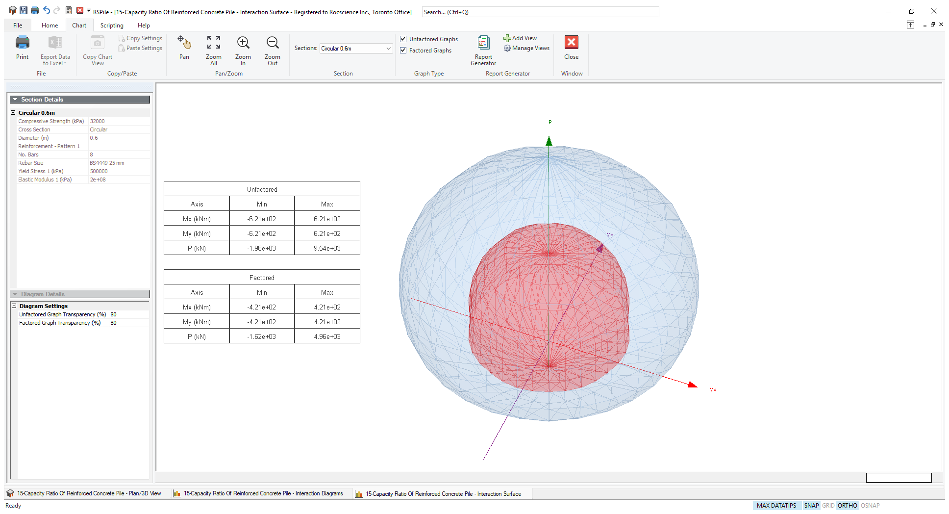
To see an animated 3D view of the unfactored or factored Interaction Surface that includes all angles and all load levels:

1. Click the 3D Interaction Surfaces icon in the Chart tab.
2. The 3D view will appear. Once again, tick the box for Factored Graphs.
3. Change the transparency level to 80% in the left panel to see the following view.