3 - Probabilistic Analysis
This tutorial familiarizes you with the Probabilistic analysis features of RocPlane.
Topics covered in this tutorial:
- Project Settings
- Probabilistic Input Data
- Probabilistic Analysis
- Histogram, Cumulative and Scatter Plots
- Random and Pseudo-Random Sampling
- Correlation Coefficient
Finished Product:
The finished product of this tutorial can be found in the Tutorial 3 Probabilistic Analysis.pln4 file, located in the Examples > Tutorials folder in your RocPlane installation folder.
1.0 Creating a New File
If you have not already done so, run the RocPlane program by double-clicking the RocPlane icon in your installation folder or by selecting Programs > Rocscience > RocPlane > RocPlane in the Windows Start menu.
When the program starts, a default model is automatically created. If you do NOT see a model on your screen:
- Select File > New

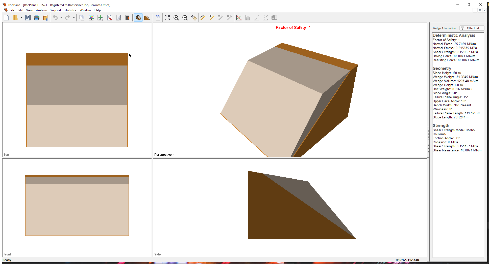
Whenever a new file is created, the default input data forms a valid wedge, as shown in the image below.
If the RocPlane application window is not already maximized, maximize it now so that the full screen is available for viewing the model.
Notice the four-pane, split screen format of the display, which shows Top, Front, Side and Perspective views of the model. This view is referred to as the 3D Wedge View. The Top, Front and Side views are orthogonal with respect to each other i.e., viewing angles differ by 90 degrees.
Before we proceed, it is very important to note the following:
- Although RocPlane displays the model in a three dimensional format, the RocPlane analysis is strictly a two-dimensional analysis. The 3D display is solely for the purpose of improved visualization of the problem geometry.
- All input data assumes that the problem is uniform in the direction perpendicular to the wedge cross-section. The analysis is performed on a “slice” through the cross-section of unit width.
- All analysis results (e.g., Wedge Weight, Wedge Volume, Normal Force, Resisting Force, Driving Force, etc.) and input data are therefore stated in terms of force per unit length, volume per unit length, etc.
2.0 Model
2.1 PROJECT SETTINGS
The Project Settings dialog allows you to configure the main analysis parameters for your model, such as Analysis Type and Units. To open the dialog:
- Select Analysis > Project Settings
 in the menu or click the icon in the toolbar.
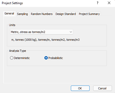
- Select the General tab,
- Set Units = Metric, stress as tonnes/m2.
- Set Analysis Type = Probabilistic.
- Select the Project Summary tab and enter RocPlane Probabilistic Analysis Tutorial as the Project Title.
- Click OK.
2.2 PROBABILISTIC INPUT DATA
Now we'll define the random variables for the Probabilistic analysis. This is done through the Probabilistic Input Data dialog. To open the dialog:
- Select Analysis > Input Data

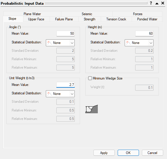
Probabilistic Input Data dialog, Slope tab - In the Slope tab, make sure Unit Weight = 2.7 t/m³.
2.2.1 Defining Random Variables
To define a random variable in RocPlane:
- Select a Statistical Distribution for the variable from the drop-down. In most cases, a Normal distribution is adequate.
- Enter Standard Deviation, Relative Minimum, and Relative Maximum values.
Any variable with Statistical Distribution = None is assumed to be exactly known and will not be involved in the statistical sampling. For more help, see Random Variables in a RocPlane Probabilistic Analysis and Overview of Statistical Distributions in RocPlane
For this tutorial, we'll define Normal Statistical Distributions for the following variables:
- Failure Plane Angle
- Failure Plane Strength Cohesion
- Failure Plane Strength Friction Angle
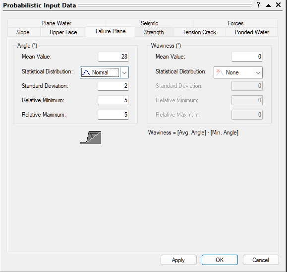
2.2.2 Failure Plane Angle
- Select the Failure Plane tab in the Input Data dialog.
- Enter the following data for the Failure Plane Angle:
- Mean Value = 28
- Statistical Distribution = Normal
- Standard Deviation = 2
- Relative Minimum = 5
- Relative Maximum = 5
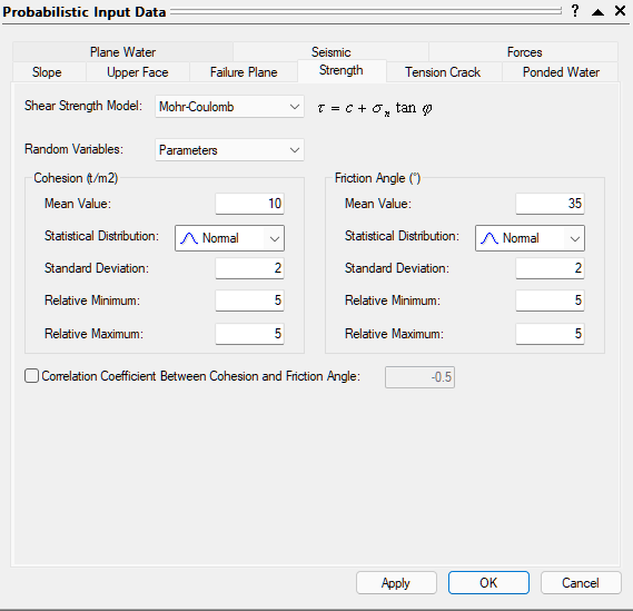
2.2.3 Failure Plane Strength Cohesion and Friction
- Select the Strength tab.
- Set Cohesion Mean Value = 10 t/m2
- Set Friction Angle Mean Value = 35 deg.
- For both Cohesion and Friction Angle, set:
- Statistical Distribution = Normal
- Standard Deviation = 2
- Relative Minimum = 5
- Relative Maximum = 5
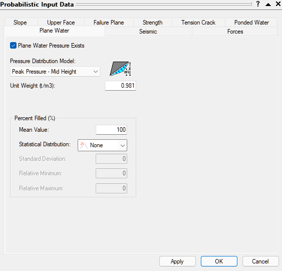
2.2.4 Water Pressure
For this tutorial, we will also apply Water Pressure.
- Select the Plane Water tab.
- Select the Plane Water Pressure Exists check box. We will use all of the default settings:
- Pressure Distribution Model = Peak Pressure – Mid Height
- Percent Filled Mean Value = 100%
- Statistical Distribution = None.
2.3 RUN THE PROBABILISTIC ANALYSIS
To carry out the RocPlane Probabilistic analysis:
- Click OK in the Probabilistic Input Data dialog.
3.0 Probabilistic Analysis
3.1 PROBABILITY OF FAILURE
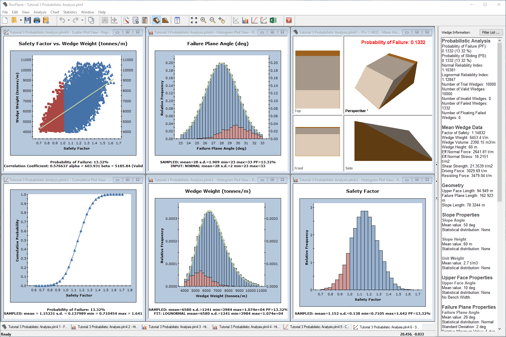
The primary result of interest from a Probabilistic analysis is the Probability of Failure. This is displayed at the top of the Perspective View in the 3D Wedge View and in the Wedge Information Panel in the Sidebar.
For this example, you should obtain a Probability of Failure of 13.3%. (i.e. PF = 0.133 means 13.3% Probability of Failure).
Later in this tutorial we'll discuss Random versus Pseudo-Random sampling. By default, Pseudo-Random sampling is in effect, which means you'll always obtain the same results each time you run a Probabilistic analysis with the same input data. With Random sampling, different results are generated each time you run the analysis. For more help, see Random Numbers Settings in RocPlane.
3.2 MEAN WEDGE DISPLAY
The wedge initially displayed after a Probabilistic analysis is based on the Mean input values and is referred to as the Mean Wedge. It appears exactly the same as the one based on Deterministic input data, with the same orientation.
Notice that the Wedge Information Panel in the Sidebar displays a Mean Wedge Data sections with the details of the wedge.
You can view other wedges generated by the Probabilistic analysis, as described in Section 3.3.2 Viewing Other Wedges below.
3.3 HISTOGRAMS
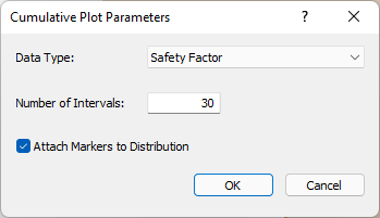
Now let's plot of a histogram of the Probabilistic analysis results, using the Histogram Plot Parameters dialog. To open the dialog:
- Select Statistic > Plot Histogram
 in the menu or click the icon in the toolbar.
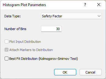 Histogram Plot Parameters dialog
 - Click OK to plot a histogram of Safety Factor.
The histogram displayed in the Histogram Plot View represents the distribution of Safety Factor for all valid wedges generated by the statistical sampling of the input. The red bars at the left of the distribution represent wedges with a Safety Factor of less than 1.0.
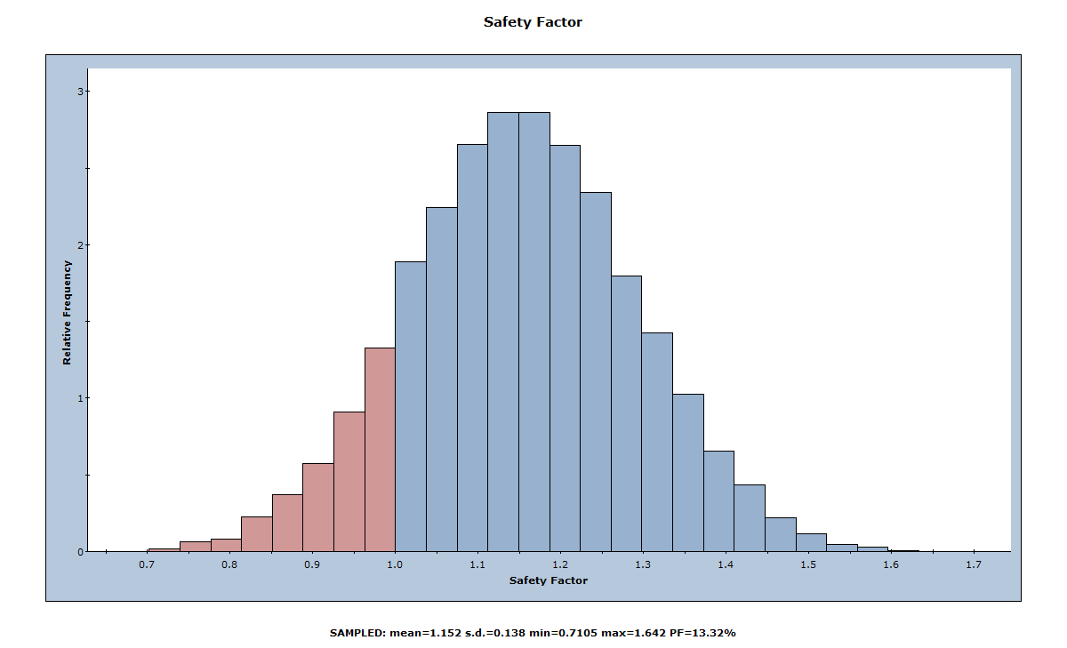
3.3.1 Mean Safety Factor
Notice the mean, standard deviation, and minimum and maximum values displayed at the bottom of the Histogram Plot View.
Note that the Mean Safety Factor from a Probabilistic analysis as shown in the Histogram Plot View (i.e., the average of all of the Safety Factors generated by the analysis) is not always the same as the Safety Factor of the Mean Wedge (i.e., the Safety Factor of the wedge corresponding to the mean input data values). You can view the Safety Factor of the Mean Wedge in the title of the 3D Wedge View or in the Mean Wedge Data section of the Wedge Information Panel in the Sidebar (press CTRL+1 to switch to the 3D Wedge View).
In this case, the two values are nearly equal (1.148 versus 1.152) because we are using Latin Hypercube sampling and 10,000 samples (see Sampling Settings in RocPlane). In general, however, these values are not equal. There are various reasons for this:
- Random sampling does not sample your input data distributions “exactly”.
- The number of samples is small.
- If invalid wedges are generated by the Probabilistic analysis, it can lead to differences between the Deterministic Safety Factor and the Probabilistic Mean Safety Factor.
3.3.2 Viewing Other Wedges ("Picked Wedge")
Now tile the Histogram Plot View and the 3D Wedge View so that both are visible.
- Select Window > Tile Vertically

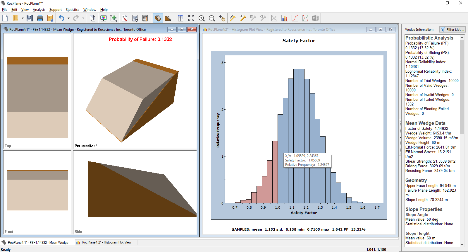
A useful feature of Histogram plots (and also Scatter plots) is the ability to view other wedges. Double-clicking on the plot displays the nearest corresponding wedge in the 3D Wedge View.
Double-click at any point along the histogram and notice that a different wedge is now displayed. Note that the Safety Factor of this wedge is displayed in the title bar of the 3D Wedge View. Also note that the title bar indicates you are viewing a Picked Wedge rather than the Mean Wedge. Double-click at various points along the Histogram and notice the different wedges and Safety Factors displayed in the 3D Wedge View. For example, click the red area of the histogram to view wedges with a Safety Factor < 1.
This feature allows you to view any wedge generated by the Probabilistic analysis corresponding to any point along the histogram distribution. In addition to the 3D Wedge View, all other views (e.g., the Info Viewer) are updated with data corresponding to the Picked Wedge.
3.3.3 Resetting the Mean Wedge
To reset all views so that the Mean Wedge data is displayed:
- Click in the wedge view
- Select Show Mean FS Wedge from the View menu
3.3.4 Histograms of Other Data
In addition to Safety Factor, you can plot histograms of the following:
- Wedge Weight, Wedge Volume
- Normal, Driving, and Resisting Forces
- Failure Plane Length, Upper Face Length
- Any random input variable (i.e., any input data variable assigned a Statistical Distribution)
For example, let's generate a histogram for Wedge Weight:
- Select Statistic > Plot Histogram
- In the Histogram Plot Parameters dialog, select Wedge Weight in the Data Type drop-down.
- Select the Best Fit Distribution check box.
- Click OK.
A histogram of the Wedge Weight distribution is generated, as shown below.
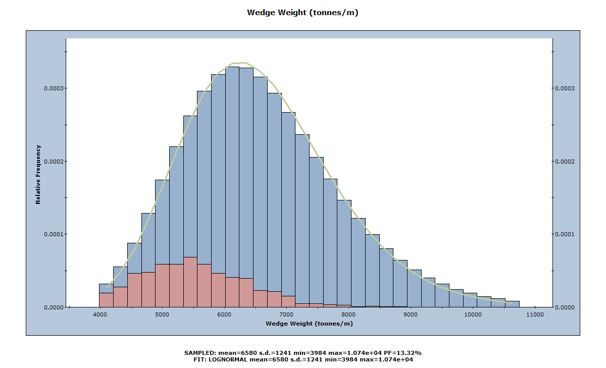
Note that all the features described above for the Histogram of Safety Factor apply to any other Data Type. For example, if you double-click on the Histogram of Wedge Weight, the nearest corresponding wedge is displayed in the 3D Wedge View.
Let's generate one more histogram. This time we'll plot one of the input data random variables: Failure Plane Angle.
- Select Statistics > Plot Histogram
- In the Histogram Plot Parameters dialog, select Failure Plane Angle in the Data Type drop-down.
- Select the Plot Input Distribution check box.
- Click OK.
The histogram shows how the Failure Plane Angle variable was sampled by the Latin Hypercube method. The curve superimposed over the histogram is the Normal distribution you defined when you entered the Failure Plane Angle Standard Deviation, Relative Minimum, and Relative Maximum values in the Input Data dialog above.
3.3.4.1 Show Failed Wedges
Notice that, on all histograms, the distribution of failed wedges (i.e., wedges with Safety Factor < 1) is automatically highlighted in red. This allows you to see the relationship between wedge failure and the distribution of any input or output variable.
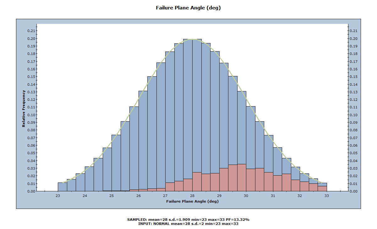
As we would expect, the failed wedges correspond to larger Failure Plane Angles, as can be seen above.
3.4 CUMULATIVE DISTRIBUTIONS (S-CURVES)
In addition to histograms, you can also plot cumulative distributions (S-curves) of the statistical results (i.e., Cumulative plots), using the Cumulative Plot Parameters dialog.
- Select Statistics > Plot Cumulative

- Click OK.
A cumulative Safety Factor distribution is generated, as shown below.
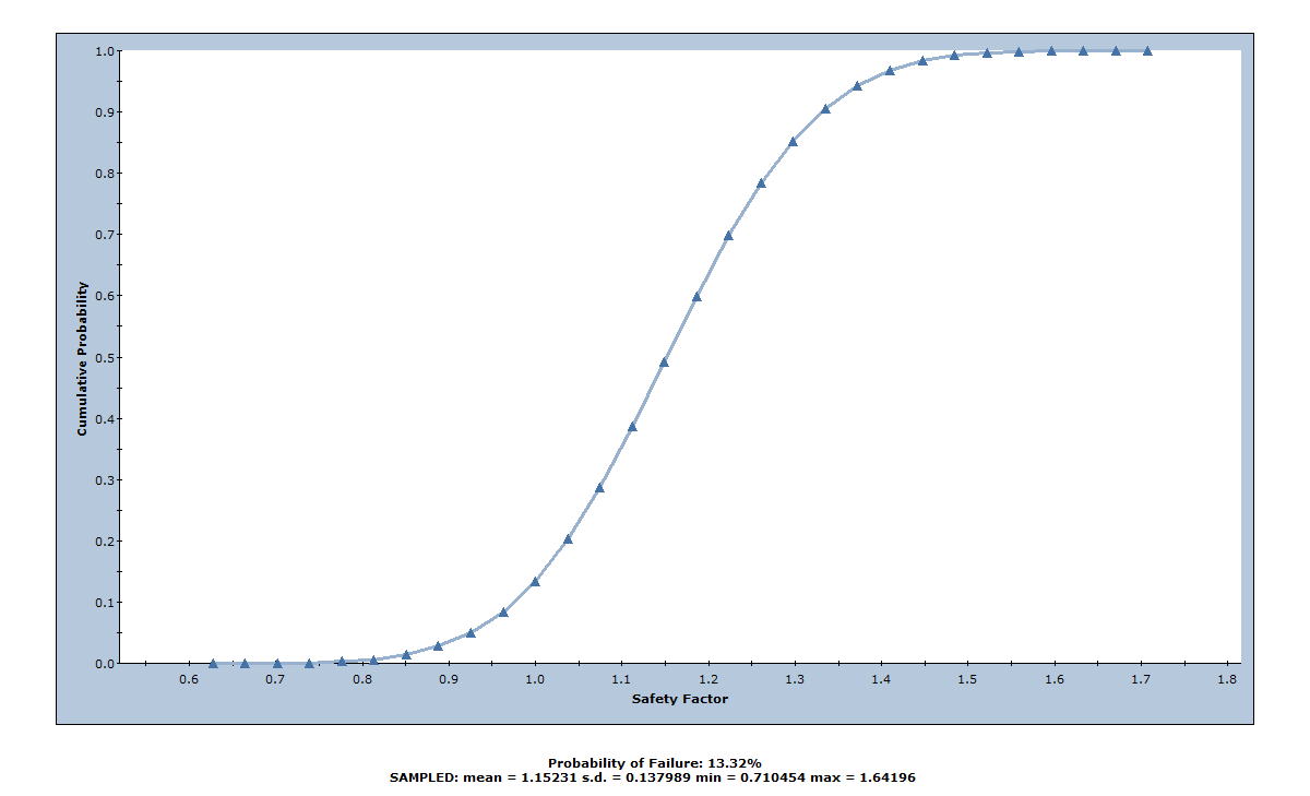
A point on a cumulative probability curve gives the probability that the plotted variable is less than or equal to the value of the variable at that point.
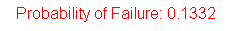
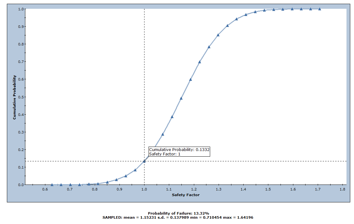
For a cumulative Safety Factor distribution, the cumulative probability at Safety Factor = 1 is equal to the Probability of Failure. We can demonstrate this with the Sampler option, which allows you to obtain the coordinates of any point on the cumulative distribution curve.
To use the Sampler option:
- On the Chart menu or right-click menu, select Sampler > Show Sampler.
You'll see a cross-hair vertical/horizontal line that follows the cursor. - Move the cursor anywhere over the cumulative probability curve to see a popup data tip that shows the Cumulative Probability and Safety Factor at that point on the curve.
- Move the cursor until you see Safety Factor = 1.
Notice that the Cumulative Probability = 0.1332, which is equal to the Probability of Failure for this example, as shown in the figure below.
- Turn off the display of the Sampler by re-selecting the Show Sampler option as above.
3.5 SCATTER PLOTS
Scatter plots allow you to examine the relationships between analysis variables. You generate a Scatter plot using the Scatter Plot Parameters dialog.
- Select Statistics > Plot Scatter

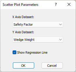
- In the Scatter Plot Parameters dialog, select the variables you want to plot on the X and Y axes. For example, Safety Factor vs. Wedge Weight.
- Select the Show Regression Line check box.
- Click OK.
As can be seen below, there appears to be very little correlation between Safety Factor and Wedge Weight. However, Safety Factor does generally increase with increasing Wedge Weight.
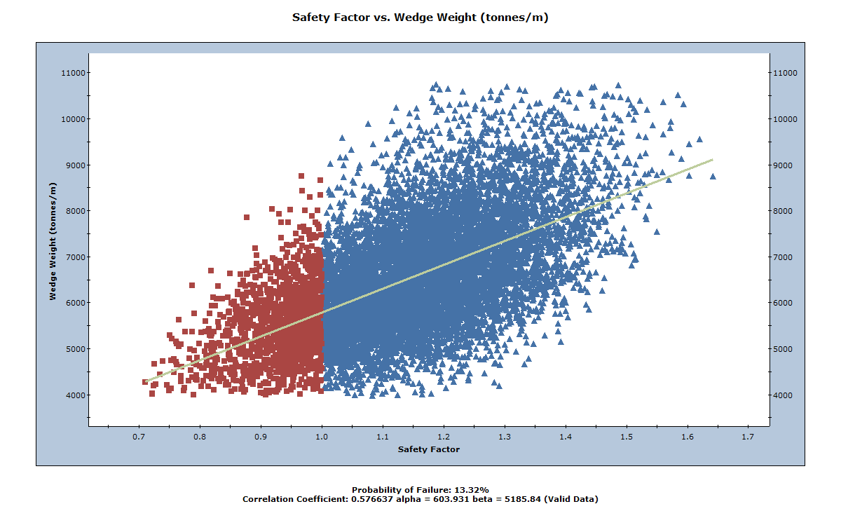
The Correlation Coefficient listed at the bottom of the plot indicates the degree of correlation between the two variables plotted. The Correlation Coefficient can vary between -1 and 1, where numbers close to zero indicate a poor correlation, and numbers close to 1 or –1 indicate a good correlation. Note that a negative Correlation Coefficient simply means that the slope of the best fit linear regression line is negative.
Alpha and beta, also listed at the bottom of the plot, represent the y-intercept and slope, respectively, of the best fit linear regression line to the scatter plot data.
NOTES:
- As demonstrated earlier with Histograms, you can double-click on a Scatter plot to display the data for the nearest wedge on the plot.
- The Show Failed Wedges option, described previously for Histograms, also works on Scatter plots. All wedges with Safety Factor < 1 are highlighted in red on the Scatter plot.
- For the special case of Cohesion vs. Friction Angle, a user-defined Correlation Coefficient can be specified in the Input Data dialog. See the Additional Exercises at the end of this tutorial for details.
4.0 Sampling Settings
4.1 RANDOM VS. PSEUDO-RANDOM SAMPLING
By default in RocPlane, Pseudo-Random sampling is in effect for a Probabilistic analysis. Pseudo-Random sampling allows you to obtain reproducible results from a Probabilistic analysis. We can demonstrate this by tiling the views.
- Select Window > Tile Vertically
Your screen should look similar to the figure below.
The Probabilistic analysis can be re-run at any time by selecting the Compute button in the toolbar.
- Select Analysis > Compute

Notice that, even though the analysis is re-run, all graphs and the Probability of Failure remain unchanged. Select Compute again to verify this.
Pseudo-Random sampling means that the SAME "seed" number is always used to generate random numbers for the sampling of the input data distributions. This results in identical sampling of the input data distributions each time the analysis is run (with the same input parameters). The Probability of Failure, Mean Safety Factor, and all other analysis output are reproducible. This can be useful for demonstration purposes or to discuss example problems.
You can change the sampling option to Random using the Project Settings dialog. The Random option uses a different seed number each time you re-compute, resulting in a different sampling of your input data distributions and therefore different analysis results.
- Select Analysis > Project Settings
- In the Project Settings dialog, select the Random Numbers tab.
- Set Random Number Generation = Random.
- Click OK.
Now re-select the Compute button several times. Notice that after each Compute:
- All graphs are updated and display new results
- The Probability of Failure is, in general, different each time the analysis is run (for this example, you should find that the Probability of Failure varies between about 13 and 14 %)
This demonstrates the difference between Random and Pseudo-Random sampling, and also graphically demonstrates the RocPlane Probabilistic analysis.
4.2 SAMPLING METHOD
So far we have used Latin Hypercube sampling throughout this tutorial. As an additional exercise, let’s try Monte Carlo sampling, with a smaller number of samples. You change this in the Project Settings dialog.
- Select Analysis > Project Settings
- In the Project Settings dialog, select the Sampling tab.
- Set Sampling Method = Monte Carlo.
- Set Number of Samples = 1000.
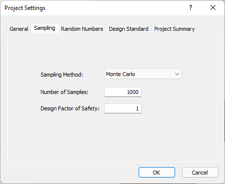
Project Settings dialog, Sampling tab - Click OK.
Examine the Probability of Failure and the Safety Factor Histogram. The results should be similar to the Latin Hypercube analysis.
The difference, as shown in the figure below, is in the sampling of the input data random variables. Notice that the Monte Carlo sampling method results in a much more variable sampling of the input data distribution compared to the Latin Hypercube method, which gives smoother results.
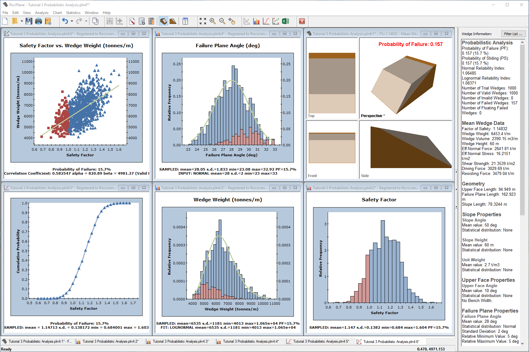
Re-compute several times and observe the variability of results each time you re-compute.
4.3 INFO VIEWER
Let’s finally examine the Info Viewer listing for a Probabilistic analysis.
- Select Analysis > Info Viewer

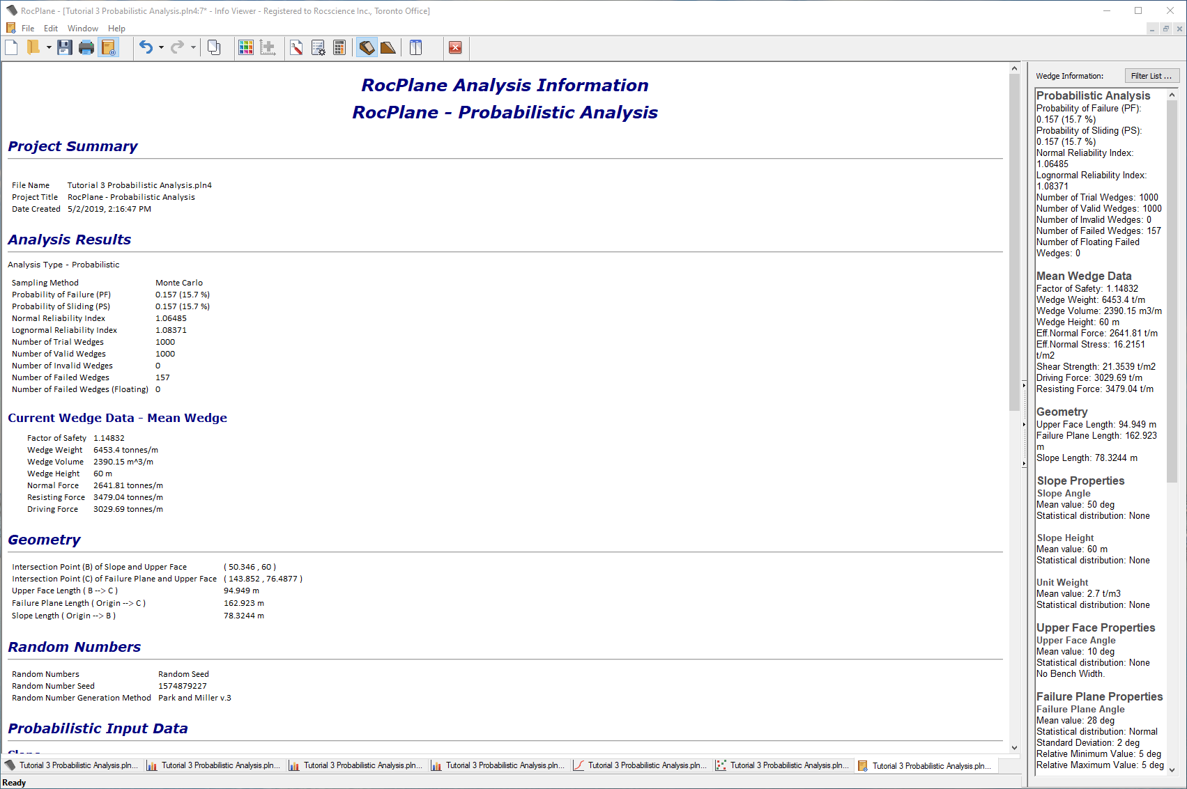
The Info Viewer displays a convenient summary of model and analysis parameters. Scroll down to view all of the information. Notice the listing of the probabilistic input and output data. As with the plot views, re-computing the analysis automatically updates the Info Viewer to reflect the latest results.
5.0 Additional Exercises
5.1 CORRELATION COEFFICIENT FOR COHESION AND FRICTION ANGLE
In this tutorial, Cohesion and Friction Angle were treated as completely independent variables. In fact, it is known that Cohesion and Friction Angle are related in a general way, such that materials with low friction angles tend to have high cohesion, and materials with low cohesion tend to have high friction angles.
You can use the Input Data dialog to define the degree of correlation between Cohesion and Friction Angle for the Failure Plane. This only applies if:
- BOTH Cohesion and Friction Angle are defined as random variables (i.e., assigned a Statistical Distribution), and
- Statistical Distribution = Normal/Uniform/Lognormal/Exponential/Gamma (will not work for Beta or Triangular).
As a suggested exercise, try the following:
- Define Normal distributions for the Cohesion and Friction Angle.
- Select the Correlation coefficient between cohesion and friction angle check box.

- Enter a Correlation Coefficient (initially, use the default value of –0.5).
- Re-run the analysis.
- Create a Scatter plot of Cohesion vs. Friction Angle.
- Note the Correlation Coefficient listed at the bottom of the Scatter plot.
It should be approximately equal to the value entered in the Input Data dialog (i.e., –0.5 in this case). - Note the appearance of the plot.
- Now repeat steps 3 to 6, using Correlation Coefficients of -0.6 to -1.0, in 0.1 increments and observe the effect on the Scatter plot.
Notice that, when the Correlation Coefficient is equal to –1, the Scatter plot results in a straight line.
5.2 EXPORTING DATA TO EXCEL
After generating any graph in RocPlane, you can easily export the data to Microsoft Excel with a single mouse click, as follows:
- Select the Chart in Excel
 button on the toolbar OR right-click on a graph and select Chart in Excel from the popup menu.
 - Export the graph data and generate a graph in Excel.
Finally, note the Export Dataset option on the Statistics menu. This option allows you to export raw data from a Probabilistic analysis to the Clipboard, a file, or Excel for post-processing. Any or all data generated by the Probabilistic analysis can be simultaneously exported.
This concludes the tutorial. You are now ready for the next tutorial, Tutorial 04 - Support in RocPlane.