17 - Statistical Plots
1.0 Introduction
This tutorial demonstrates the use of statistical plots (e.g., Plot Histogram, Plot Scatter, Plot Cumulative) to fit distributions and perform linear regression on quantitative Grid Data.
Topics Covered in this Tutorial:
- Grid Data
- Histogram Plot and Best Fit Distribution
- Scatter Plot and Regression Line
- Cumulative Plot
Finished Product:
The finished product of this tutorial can be found in the Tutorial 17 Statistical Plots.dips8 file, located in the Examples > Tutorials folder in your DIPS installation folder.
2.0 Model
If you have not already done so, run DIPS by double-clicking on the DIPS icon in your installation folder. Or from the Start menu, select Programs > Rocscience > DIPS > DIPS.
If the DIPS application window is not already maximized, maximize it now, so that the full screen is available for viewing the model.
DIPS comes with several example files installed with the program. These example files can be accessed by selecting File > Recent Folders > Examples Folder from the DIPS main menu. This tutorial will use the Orthogonal Sets.dips8 file to demonstrate the basic plotting features of DIPS.
- Select File > Recent Folders > Example Folder
 from the menu.
 - Open the Orthogonal Sets.dips8 file. Since we will be using the Orthogonal Sets.dips8 file in other tutorials, save this example file with a new file name without overwriting the original file.
- Select File > Save As
 from the menu.
 - Enter the file name Tutorial 17 Statistical Plots and Save the file.
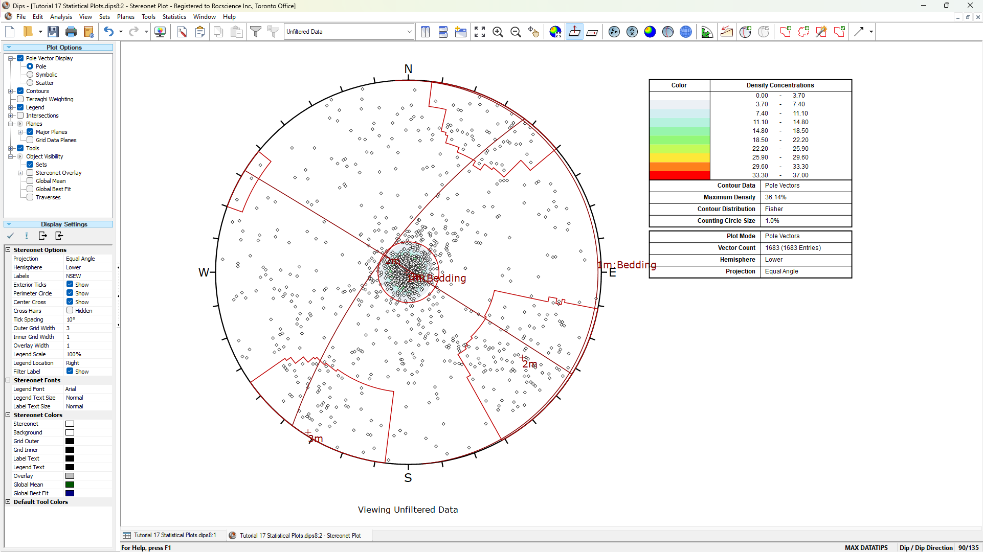
You should see the Stereonet Plot View shown in the following figure.
- Switch to the Grid Data view of the file using the view tabs in the lower left of the window.
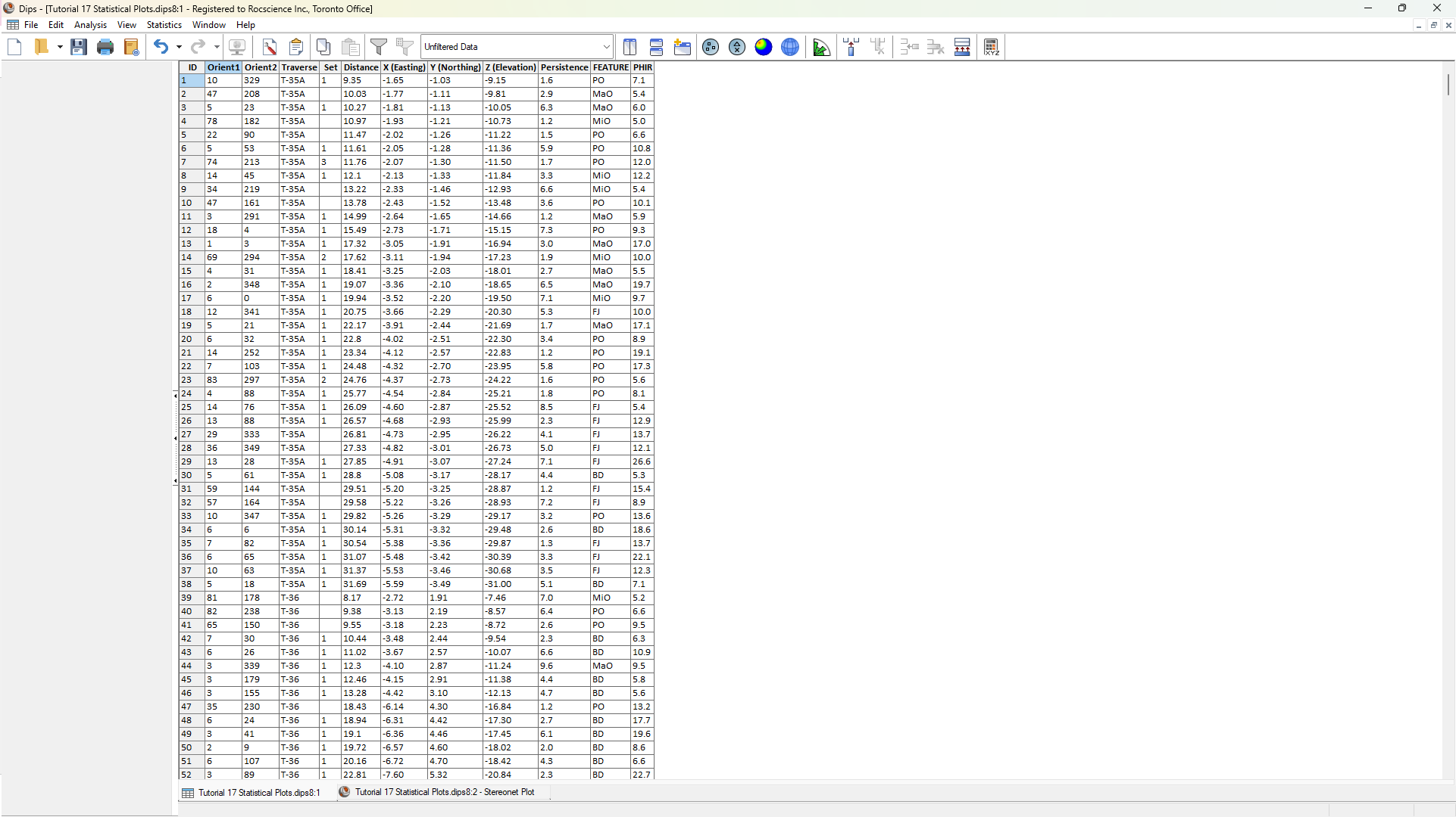
The file contains 1683 measurements from 47 televiewer linear borehole cores.
The file uses the following columns:
- The two mandatory Orientation columns
- A Traverse column
- A Set column
- A Distance column
- Three location X, Y, Z columns
- A Persistence columns
- 2 extra columns
3.0 Statistical Plots
In DIPS, statistical plots (e.g., histogram plot, scatter plot, cumulative plot) can be generated for any quantitative column in the Grid Data.
3.1 Histogram Plot
A histogram plot is a graphical representation that displays the distribution of a dataset. It consists of a series of bars, where the height of each bar corresponds to the frequency or relative frequency of data falling within a particular interval or bin. A statistical distribution can also be fitted to the dataset. The following distributions are available in DIPS:
To plot a histogram of Persistence:
- Select Statistics > Plot Histogram
 from the menu .
 - In the Histogram Plot Parameters dialog:
- Set the Data Type = Persistence.
- Enter Number of Intervals = 30.
- Select Attach Markers to Distribution checkbox.
- Select Best Fit Distribution (Kolmogorov-Smirnov Test) checkbox to fit a distribution to the data.
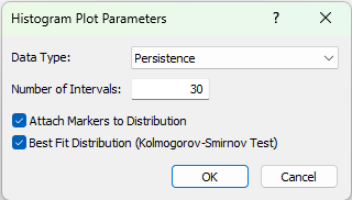
Histogram Plot Parameters with Dataset set to Persistence - Click OK to generate the histogram plot.
The Histogram Plot view shows the Relative Frequency on the y-axis and Persistence on the x-axis. The Best Fit Distribution is fit with an Exponential Distribution through the data.
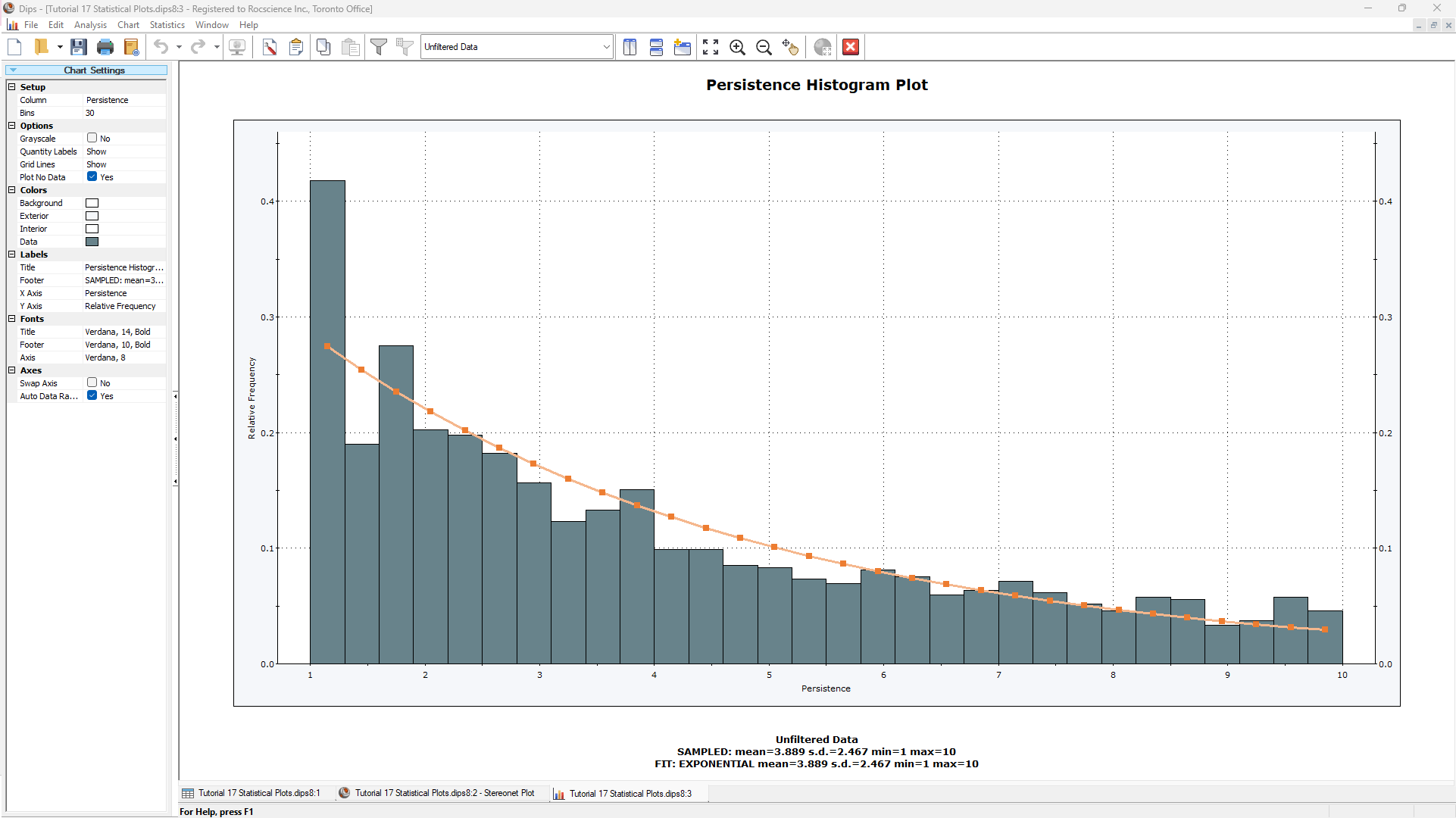
The SAMPLED and FIT distributions show the following:
- Mean = 3.889
- Standard Deviation = 2.467
- Min = 1
- Max = 10
3.2 Scatter Plot
A scatter plot is a graphical representation that displays the relationship between two variables. A linear regression can be fitted through the dataset to see if there is a correlation between the two variables plotted.
To plot a scatter plot of Z (Elevation) vs PHIR:
- Select Statistics > Plot Scatter
 from the menu .
 - In the Scatter Plot Parameters dialog:
- Set the X Axis Dataset = Z (Elevation).
- Set the Y Axis Dataset = PHIR.
- Select Show Regression Line checkbox to fit a linear regression through the data.
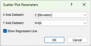
Scatter Plot Parameters dialog with X Axis Dataset set to Z (Elevation) and Y Axis Dataset set to PHIR - Click OK to generate the scatter plot.
The Scatter Plot view shows the Z (Elevation) values on the x-axis vs. PHIR values on the y-axis. The Regression Line is fit through the data.
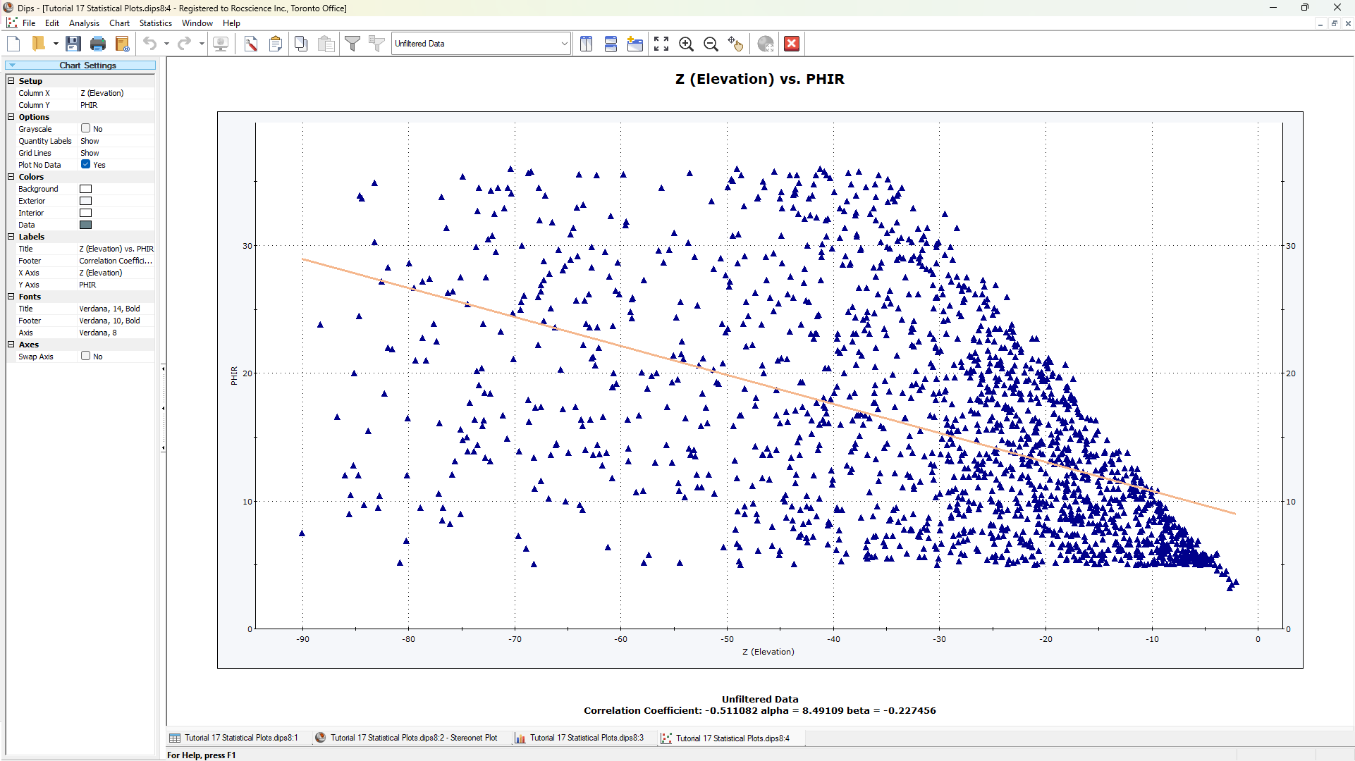
The residual friction angle (i.e., PHIR) is loosely negatively correlated with the Z (Elevation) as indicated by the Correlation Coefficient of -0.511. The alpha and beta values represent the y-intercept and slope of regression line, respectively.
3.3 Cumulative Plot
A cumulative plot is a graphical representation that shows the cumulative distribution of a dataset.
To plot a cumulative plot of Processed Dip:
- Select Statistics > Plot Cumulative
 from the menu.
 - In the Cumulative Plot Parameters dialog:
- Set the Data Type = Processed Dip.
- Enter Number of Intervals = 30.
- Select the Attach Markers to Distribution checkbox.
- Click OK to generate the cumulative plot.
NOTE: In this example, Orient 1 and Processed Dip are equivalent since all measurements are either Dip/Dip Direction according to the Global Orientation or recorded along a Linear BH Televiewer Traverse with Dip/Dip Direction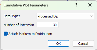
Cumulative Plot Parameters dialog with Data Type set to Processed Dip
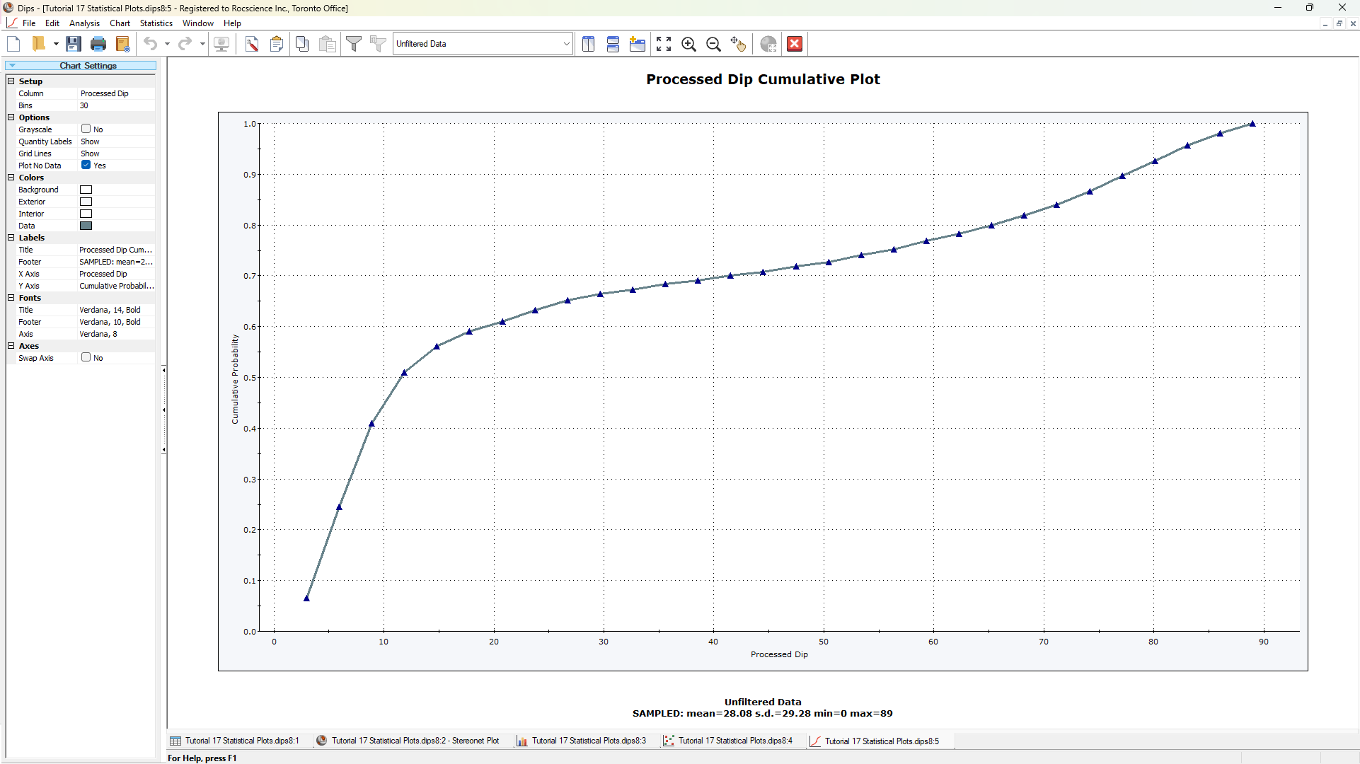
The Cumulative Plot view shows the Cumulative Probability values on the y-axis and Processed Dip on the x-axis.
To view a subset of the data, we can apply a filter to the Cumulative Plot View.
- From the Filter drop down in the toolbar, select the Bedding filter.
Only data in the Bedding filter will be used to generate the cumulative plot.
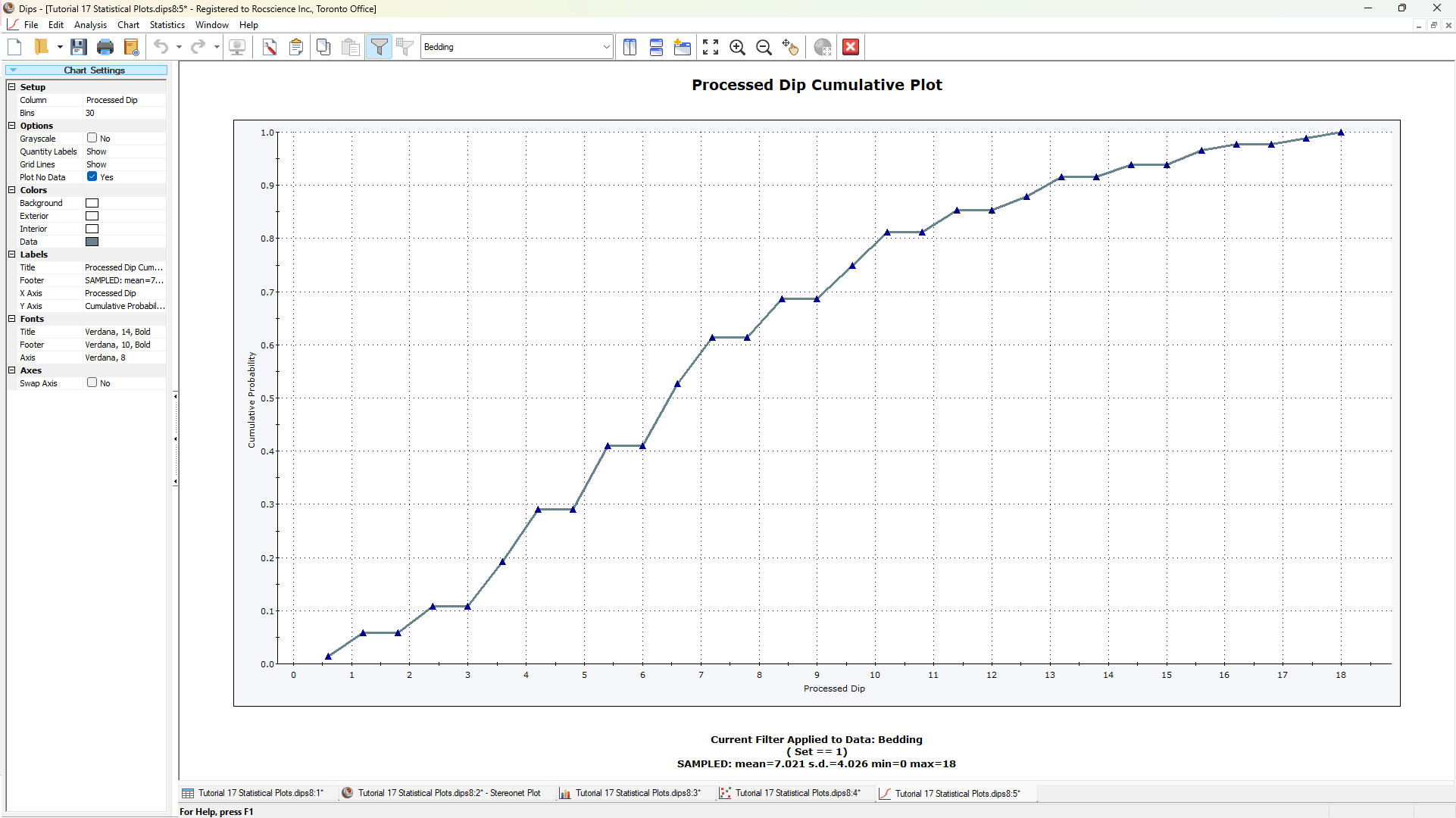
The footer at the bottom of the chart indicates that the Current Filter Applied to Data is the Bedding filter, which includes all poles in Set 1.
This concludes the tutorial.