10 - Kinematic Analysis (Wedge Sliding)

1.0 Introduction

Based on kinematic considerations and frictional properties of joint planes, it is possible to perform stability analyses such as toppling, Planar Sliding and Wedge Sliding on a stereonet. This tutorial demonstrates how to perform stability analyses under Wedge Sliding failure mode using the Kinematic Analysis option in Dips.

The tutorial is a continuation from Tutorial 07 - Feature Analysis (which uses the example file Examppit.dips8) . The data has been collected by a geologist working on a single rock face above the first bench in a young open pit mine.

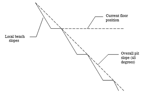
The rock face above the current floor of the existing pit has a dip of 45 degrees and a dip direction of 135 degrees. The current plan is to extend the pit down at an overall angle of 45 degrees. This will require a steepening of the local bench slopes, as indicated in the figure above. The local benches are to be separated by an up-dip distance of 16m. The bench roadways are 4m wide.

Topics Covered in this Tutorial:

• Kinematic Analysis of Wedge Sliding Failure Mode
• Friction Cones
• Intersections
• Sensitivity Analysis

Finished Product:

The finished product of this tutorial can be found in the Tutorial 10 Kinematic Analysis (Wedge Sliding).dips8 file, located in the Examples > Tutorials folder in your Dips installation folder.

2.0 Model

If you have not already done so, run Dips by double-clicking on the Dips icon in your installation folder. Or from the Start menu, select Programs > Rocscience > Dips > Dips.

If the Dips application window is not already maximized, maximize it now, so that the full screen is available for viewing the model.

To save us some time, this tutorial will use the Tutorial 07 Feature Analysis.dips8 file which already has the required pit slope plane (User Plane) and .

1. Select File > Recent Folders > Tutorials Folder from the menu.
2. Open the Tutorial 07 Feature Analysis.dips8 file. Save this example file with a new file name without overwriting the original file.
3. Select File > Save As from the menu.
4. Enter the file name Tutorial 10 Kinematic Analysis (Wedge Sliding) and Save the file.

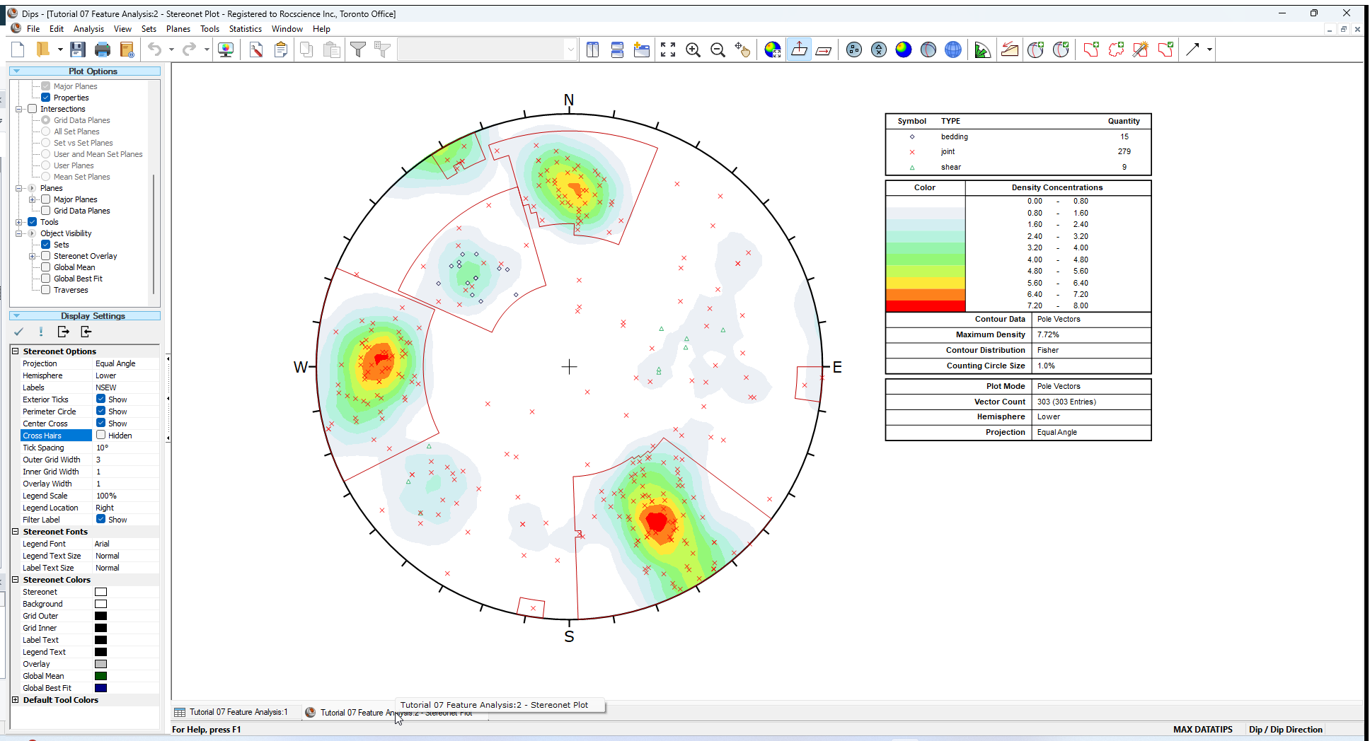
You should see the Stereonet Plot View shown in the following figure.

If you do not see the plot below, then use the Sidebar Plot Options to view pole vectors and contours on the stereonet.

3.0 Wedge Sliding

From the Planar Sliding Kinematic Analysis, it has been shown that a sliding failure along any single joint plane is unlikely. However, multiple joints can form wedges which can slide along the line of intersection between two planes.

1. Select the Kinematic Analysis option from the Analysis menu.
2. In the Kinematic Analysis dialog:
1. Select Display Kinematic Analysis checkbox.
2. Set the Failure Mode = Wedge Sliding in the dropdown.
3. Enter Slope Dip = 45 degrees.
4. Enter Slope Dip Angle = 135 degrees.
5. Enter Friction Angle = 30 degrees.



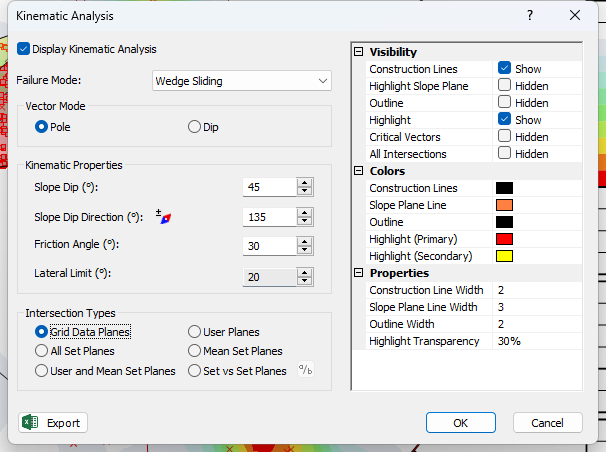
6. Select OK.

Also do the following:

3. Turn off the display of pole vectors (unselect the Pole Vector Display checkbox in the Sidebar Plot Options).
4. Turn on the display of Intersection Contours (select Contours > Intersection in the Sidebar Plot Options).

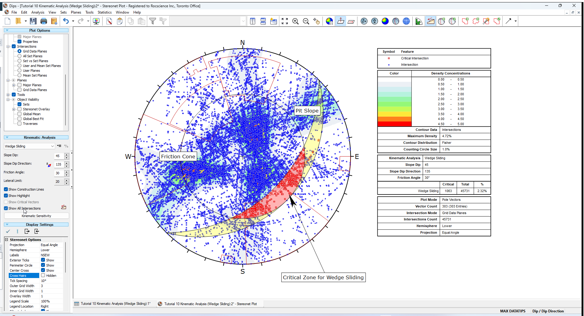
You should see the Kinematic Analysis overlay for Wedge Sliding as shown below.

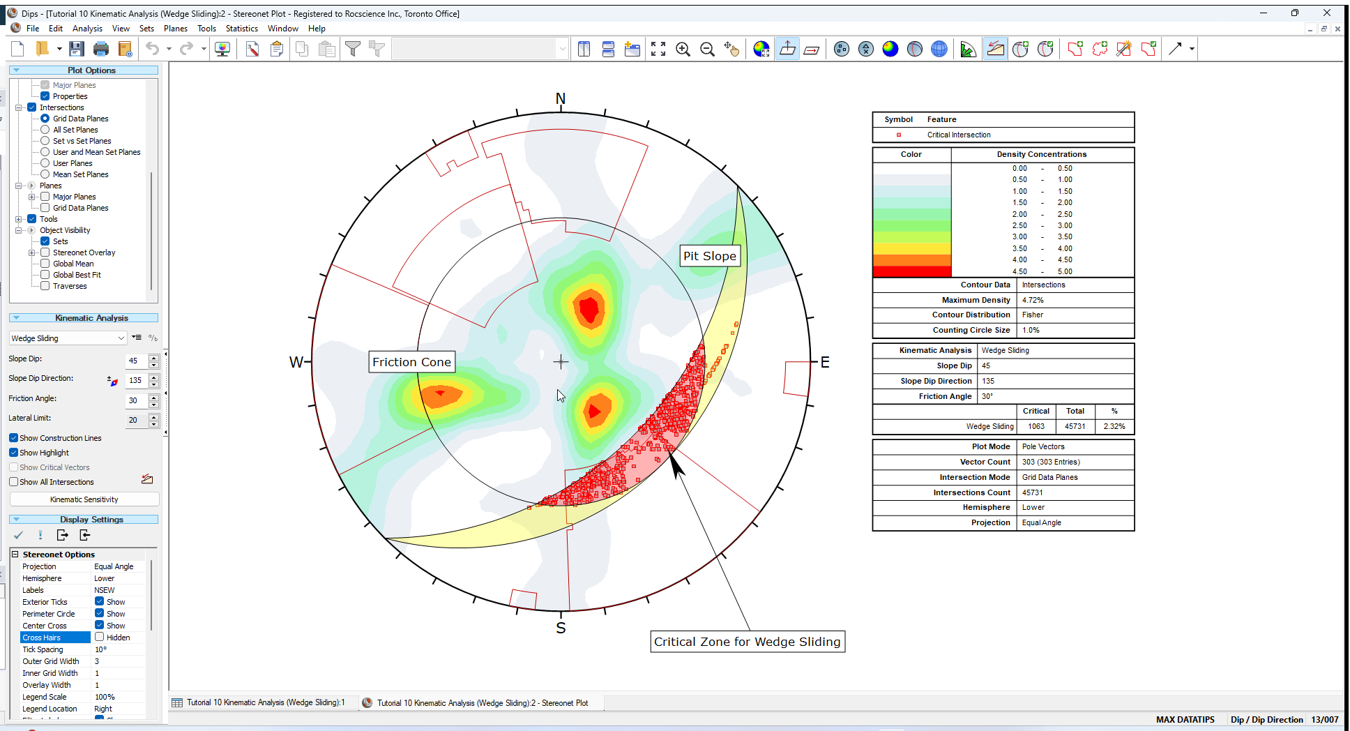
The key elements of Wedge Sliding analysis are:

• Slope Plane
• Plane Friction Cone (angle measured from perimeter of stereonet)
• Intersection plotting

The Primary Critical Zone for Wedge Sliding is the crescent shaped area INSIDE the Plane Friction Cone and OUTSIDE the Slope Plane. Any intersection points that plot within this zone represent wedges which are able to slide.

3.1 INTERSECTIONS

The points that you see plotted for the Wedge Sliding analysis are intersection points. Each point represents the intersection of two joint planes. By default, all planes in the file are considered (i.e. each plane in the file is intersected with every other plane in the file, to determine the intersection points). The intersection points represent the actual Trend/Plunge of the line of intersection of two joint planes. By default only the critical intersections are displayed.

There are several options available for the display of intersections:

• All planes in the file can be intersected with each other (Grid Data Planes option).
• Intersection contours can be displayed (based on the intersection of all planes) as shown above.
• Major plane intersections can be plotted (i.e., Mean Set Planes and/or User Planes).

3.2 INTERSECTION CONTOURS

An immediate indication that Wedge Sliding is not an issue for this slope orientation, are the intersection contours. You can see that the main concentrations of intersections are all well outside the Critical Zones for Wedge Sliding.

3.3 SLOPE PLANE

The pit slope plane defines the daylighting condition for intersections. Any intersection point which plots outside the pit slope great circle (i.e., intersection vector plunges below the pit slope plane) satisfies the daylighting condition.

3.4 FRICTION CONE

For Wedge Sliding, it is important to remember that the friction cone (30 degrees) is measured from the EQUATOR of the stereonet, and NOT FROM THE CENTER, because we are dealing with an actual sliding surface or line. (When we are dealing with poles the friction cone is measured from the center of the stereonet).

3.5 CRITICAL ZONE FOR WEDGE SLIDING

The Primary Critical Zone for Wedge Sliding is the crescent shaped area INSIDE the plane friction cone and OUTSIDE the slope plane (highlighted in red in the above figure). Intersections which plot in this zone represent wedges which satisfy frictional and kinematic conditions for sliding.

However wedges do not necessarily slide along the line of intersection of two joint planes. Wedges can slide on a single joint plane, if one plane has a more favourable direction for sliding than the line of intersection. In this case, the second joint plane acts as a release plane rather than a sliding plane. This can occur in either the primary or the secondary critical region.

The Secondary Critical Zone (highlighted in yellow in the above figure) is the area between the slope plane and a plane (great circle) inclined at the friction angle. Critical intersections which plot in these zones always represent wedges which slide on one joint plane. In this region, the intersections are actually inclined at LESS THAN the friction angle, but sliding can take place on a single joint plane which has a dip vector greater than the friction angle.

4.0 Results Legend

A summary of the Wedge Sliding results is displayed in the Legend.

For this example, the percentage of critical intersections compared to the total number is actually very low (about 2 percent) so Wedge Sliding is not a great concern for this slope orientation.

5.0 Intersections

To view all intersections:

1. Select the Show All Intersections checkbox in the Kinematic Analysis options in the Sidebar.

This will give you a better feel for the relatively small number of critical intersections compared to the total number, as shown below.

5.1 MEAN SET PLANE INTERSECTIONS

Let’s demonstrate one more possibility for assessing the risk of Wedge Sliding. We will view the intersections of the Mean Set Planes (from the four sets we created earlier in this tutorial).

1. Select Intersections > Mean Set Planes in the Sidebar Plot Options.
2. Select Planes > Major Planes > Mean Set Planes in the Sidebar Plot Options to display the Mean Set Planes.

The plot should look as follows.

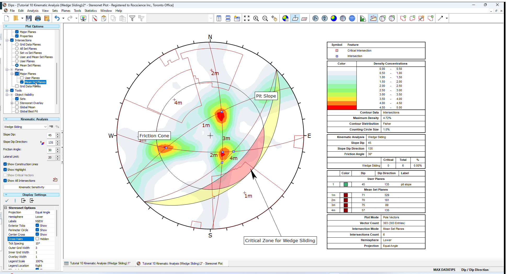
Notice that the four Mean Set Planes intersect each other to form 6 intersection points. Notice that these intersections correspond with the maximum concentrations of the intersection contours, as we would expect.

Since none of the Mean Set Plane intersections are within the Critical Wedge Sliding Zone, again we can conclude that Wedge Sliding is not an issue for this slope orientation. Note that the Legend indicates zero critical intersections out of a total of 6 Mean Set Plane intersections.

5.2 DISCRETE STRUCTURES

Finally, for Wedge Sliding you should analyze the shear zones (TYPE = shear). If these shears occur in proximity to one another they may interact to create local instability.

Perform an analysis similar to the one above using discrete combinations of shear planes.

• Use the Add User Plane option to add planes corresponding to the shear features.

TIP: While using Add User Plane, the Pole Snap option (available in the right-click menu) can be used to snap to the exact orientations of the shear poles.

Determine whether the shears will interact with any of the mean joint set orientations to create an unstable wedge. Using the procedure described above, the stability of discrete combinations of shear planes, or of shear planes with the mean joint orientations, may be analyzed. In the Sidebar plot options, select Intersections > User Planes (or Intersections > User and Mean Set Planes).

You should find that the risk of wedge failure along the shear planes is low, for this pit slope configuration.

We will leave this as an optional excercise.

Switch back to display of all intersections:

1. Select Intersections > Grid Data Planes in the Sidebar Plot Options.
2. Unselect Planes > Major Planes > Mean Set Planes in the Sidebar Plot Options to turn off the display of Mean Set Planes.
3. Unselect Show All Intersections checkbox in Sidebar Kinematic Options.

6.0 Terzaghi Weighting

It is important to note the effect of the Terzaghi Weighting on the Kinematic Analysis results.

• If the Terzaghi Weighting checkbox is selected in the Sidebar Plot Options, the effect of bias correction on the Kinematic Analysis results will be accounted for and the Kinematic Analysis results will be reported in terms of weighted counts of poles or intersections.
• The weighting is applied to each pole based on the angle between the plane and the Traverse on which the data was collected, and all pole counts and “critical percent” values for all failure modes, are reported using the weighted count values.
• Weighting is only applicable for data collected on Traverses.

Turn on Terzaghi Weighting:

1. Select Terzaghi Weighting checkbox in the Sidebar Plot Options.

The weighting affects the critical count, the total count and the percent critical value for the Kinematic Analysis, for poles and for intersections (used for Wedge Sliding and Direct Toppling modes) and is reported in the Legend when weighting has been applied.

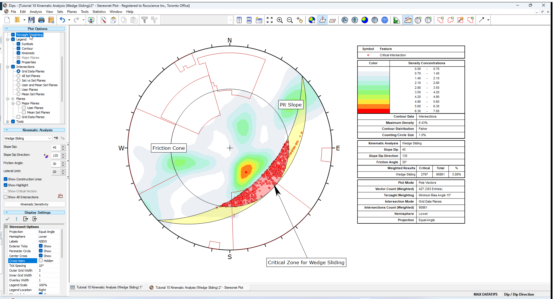
Whenever you use Terzaghi Weighting you should understand the significance of the weighting method and its application to design. If the Terzaghi Weighting checkbox is turned OFF, then the kinematic results will be based on the raw pole counts with no bias correction.

2. Toggle the Terzaghi Weighting checkbox to see the effect of applying bias correction to the Mean Set Planes. The effect in this case is small.

7.0 Info Viewer

Although the Legend displays a summary of Kinematic Analysis results for the currently selected method, the Info Viewer provides a detailed summary of kinematic results for ALL failure modes.

As soon as Kinematic Analysis is enabled, Dips automatically carries out the analysis behind the scenes, for all failure modes, for the current input parameters (slope orientation, friction angle, lateral limits) and this information is available at all times in the Info Viewer.

1. Select Info Viewer from the toolbar or the Analysis menu.
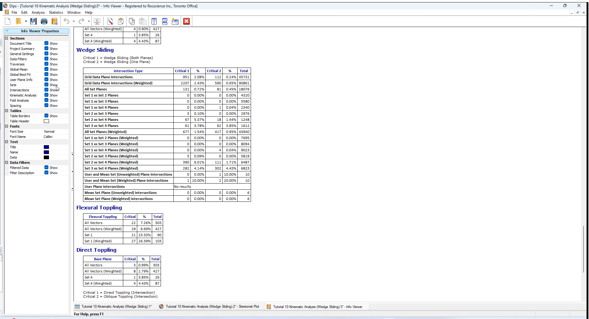
2. Scroll down to the Kinematic Analysis section of the Info Viewer to see the results for all failure modes.

7.1 WEDGE SLIDING

The Info Viewer reports both weighted and unweighted results together, so that you can easily compare results and see the effect of the weighting.

For further details see the Dips Info Viewer topic.

8.0 Sensitivity Analysis

The Kinematic Sensitivity option in Dips makes it easy to perform sensitivity analysis, by varying the main input parameters (Slope Angle, Slope Dip Direction, Friction Angle) and plotting the results for each failure mode. As noted above, results for all failure modes are always available in the Info Viewer.

8.1 INCREASED LOCAL PIT SLOPE

Let's see the affect of steeper local slopes. If the overall slope is to be maintained at 45 degrees, the local bench slope will have to be increased to accommodate the roadways. What is the critical local slope?

8.2 OTHER PIT ORIENTATIONS

Assume that the joint sets are consistent throughout the mine property. Are there any slope orientations that are more unstable than others? Use the Kinematic Sensitivity option to examine slope dip direction in +/- 45 degrees around the pit wall.

To perform a Kinematic Sensitivity Analysis:

1. Go back to the Stereonet Plot view.
2. Select Kinematic Sensitivity from the Analysis menu (or alternatively, the Kinematic Sensitivity button in the Sidebar Kinematic Analysis).
3. In the Kinematic Sensitivity dialog:
1. Keep the Failure Mode = Wedge Sliding.
2. Select the Slope Dip checkbox.
3. Set the Slope Dip range From = 45 degrees, To = 90 degrees, at Interval = 1 degrees.
4. Select the Slope Dip Direction checkbox.
5. Set the Slope Dip range From = 90 degrees, To = 180 degrees, at Interval = 1 degrees.



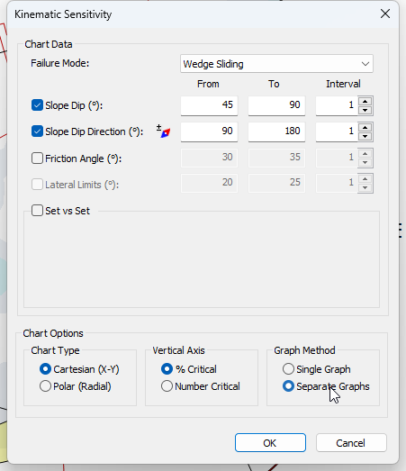
6. Set Graph Method = Separate Graphs.
7. Select OK to generate the plot.

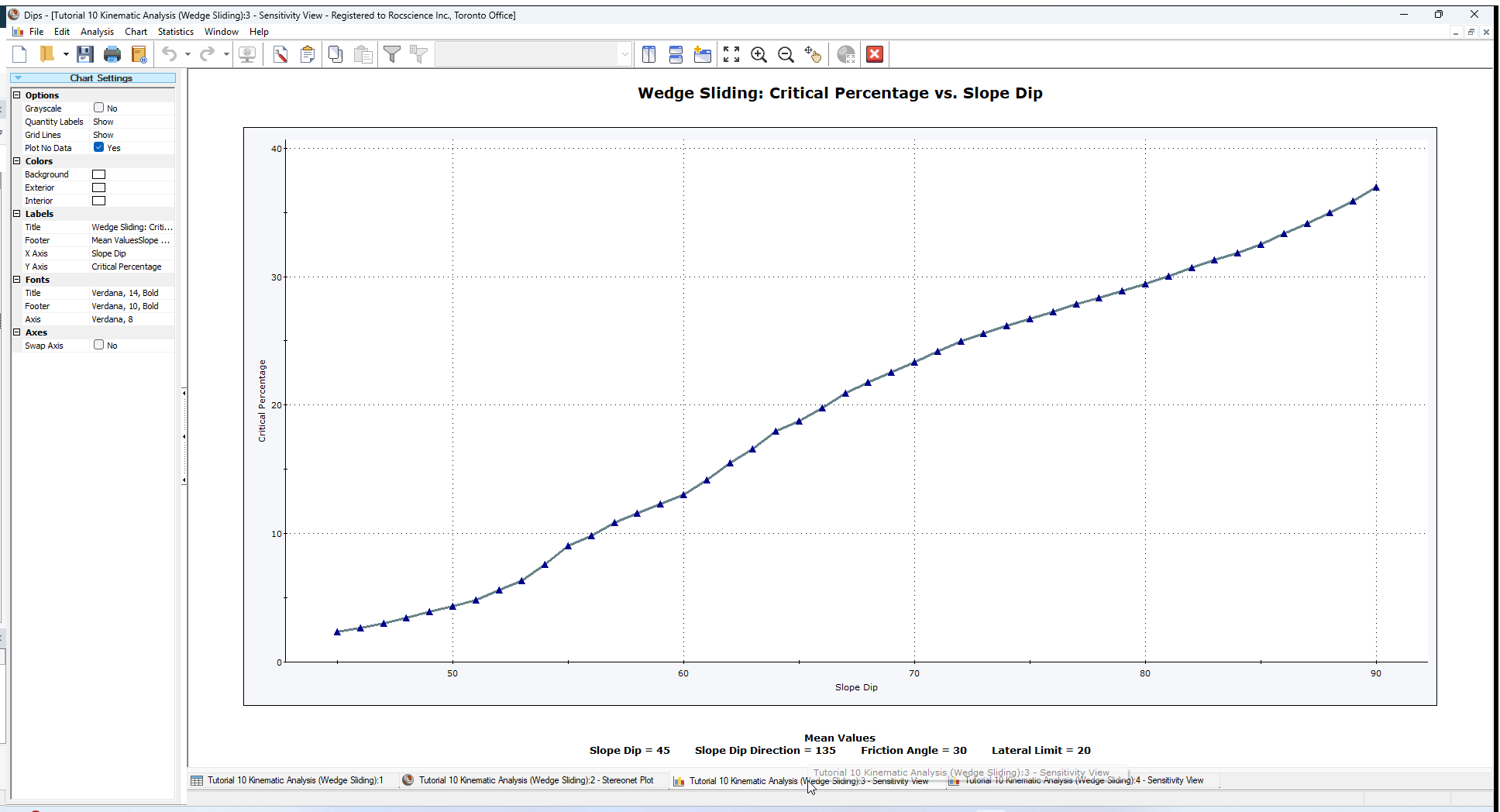
From examining the Sensitivity Plots, we get an increase in the percentage of possible Kinematic Wedge Sliding failures as the Slope Dip becomes steeper.

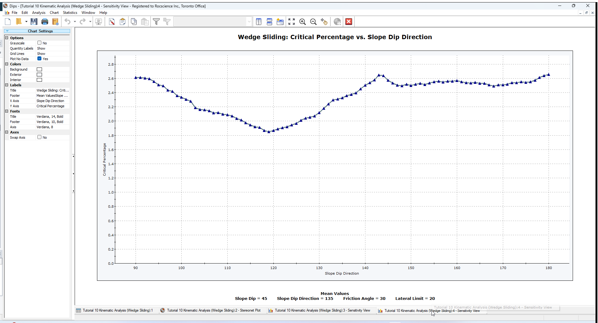
The Slope Dip Direction has very little affect on the percentage of possible Kinematic Wedge Sliding failures (below 3%).

NOTE:

• You can import Dips plots into AutoCAD using the Copy Metafile option in the Edit menu. This will copy a metafile of the current view to the clipboard, which can then be pasted into AutoCAD.
• Pole or Contour plots showing mean planes and the selected pit slope orientation can be imported into a plan of the pit and placed in their appropriate orientations for quick reference.

9.0 Summary

Kinematic Analysis of rock slope failure modes using stereonets is an extremely useful and easy to understand analysis tool which allows you to quickly evaluate potential failure modes. However keep in mind the following.

• The analyses presented here are just a starting point for more detailed analysis and should always be accompanied by a more thorough field analysis in cases where a risk of failure is indicated.
• Real slopes may exhibit more than one failure mode. It is rare to see pure examples of these failure modes, particularly with the toppling analysis, which may exhibit complex behaviours involving sliding, toppling, rotating etc.
• Even if a Kinematic Analysis indicates risk of failure, this does not necessarily mean that failure will occur, since factors other than kinematics and friction angle may work to increase stability (e.g. joint cohesion, joint persistence etc). Conversely, other factors may decrease stability (e.g. water pressure) of kinematically safe slopes.
• It is important to look beyond statistical results (e.g. mean set plane orientations) and consider major discrete structures such as shear zones which may have a dominant effect on stability due to low friction angles and inherent persistence.
• More detailed analysis including safety factor calculation can be carried out with the Rocscience programs SWedge (wedge analysis), RocPlane (planar analysis) and RocTopple (toppling analysis).

10.0 References

1. Goodman, R.E. 1980. Introduction to Rock Mechanics (Chapter 8), Toronto: John Wiley, pp 254-287.
2. Hudson, J.A. and Harrison, J.P. 1997. Engineering Rock Mechanics – An Introduction to the Principles, Pergamon Press.

This completes the tutorial. You are now ready for the next tutorial, Tutorial 11 - Oriented Core and Rock Mass Classification in Dips.