2 - Synthetic Joint Sets
1.0 Introduction
Joint sets are groups of joints which have similar orientation. Using distributions of joint set orientation, spacing, and size, we can statistically sample and generate joints across a provided traverse (i.e., scanline, borehole, etc.). This tutorial covers the use of synthetic joints in RocSlope3.
Finished Product
The finished product of this tutorial can be found in the Tutorial 02 Synthetic Joint Sets folder. All tutorial files installed with RocSlope3 can be accessed by selecting File > Recent Folders > Tutorials Folder from the RocSlope3 main menu.
2.0 Opening the Starting File
- Select File > Recent > Tutorials Folder in the menu.
- Go to the Tutorial 02 Synthetic Joint Sets folder and open the starting file Tutorial 02 Synthetic Joints Sets - starting file.rocslope_model.
This model already has the following defined and provides a good starting point to start defining synthetic joint sets:
- Project Settings
- Material Properties
- External Geometry
2.1 Project Settings
Review the Project Settings.
- Select Analysis > Project Settings

- Select the Units tab. Ensure Units are Metric, stress as
MPa.
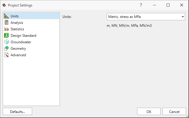
Unit tab in Project Settings Dialog - Select the Analysis tab.
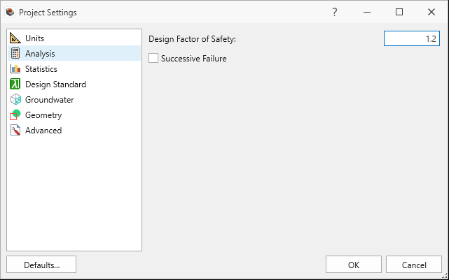
Analysis tab in Project Settings Dialog - Ensure Successive Failure = OFF. We will only be analyzing the blocks which daylight and are readily removable.
- Set Combined block (computes largest removable) = OFF. We will only be analyzing unit blocks in this tutorial.
- Ensure Design Factor of Safety = 1.2.
- Select the Statistics tab.
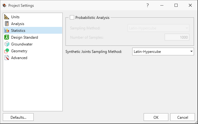
Statistics tab in Project Settings Dialog - Ensure Synthetic Joint Sampling = Latin Hypercube and keep everything else as default.
- Click OK to close the dialog.
2.2 Material Properties
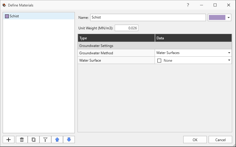
Review the Material Properties.
- Select Materials > Define Materials

- One (1) material property is defined. The Schist material property has:
- Unit Weight = 0.026 MN/m3.
- No Water Surface applied.
2.3 External Geometry
The External is of a pit shell and is composed of one volume assigned with the Schist material property.
3.0 Defining Joint Properties
- Navigate to the Joints workflow tab

- Select Joints > Define Joint Properties

The Define Joint Properties dialog will open. This dialog allows users to define the Strength Model, Waviness, and Water Pressure for each joint property.
- Enter the following properties for Joint Property 1:
- Name = Smooth
- Under the Strength tab:
- Strength Model = Mohr-Coulomb
- Cohesion = 0 MPa
- Phi = 10 deg
- Override by Material = OFF
- Waviness = 0 deg
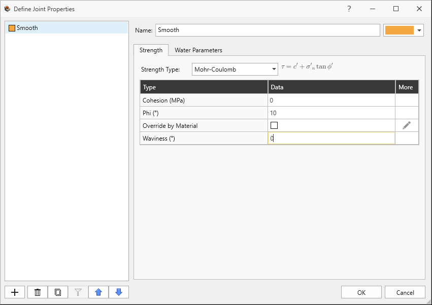
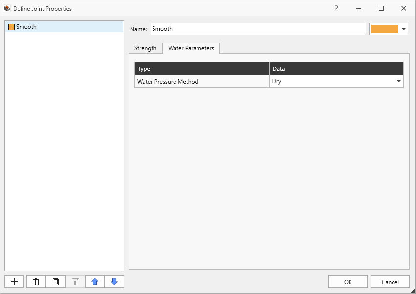
Smooth Joint Property Strength tab in Define Joint Properties Dialog - Under the Water Parameters tab:
- Water Pressure Distribution = Dry
4.0 Adding Synthetic Joints
In this example, we will be defining synthetically joints sampled using set statistics data from DIPS. For a given Synthetic Joint Property, the following distributions are specified:
- Orientation (i.e., dip and dip direction)
- Spacing (i.e., distance between adjacent joints in a set)
- Radius
With the orientation, spacing, and radius distributions, the user then defines the traversal path as a polyline on which the X, Y, Z center location of each joint is sampled, according the the spacing. For each joint, the orientation and radius is sampled according to their respective distributions. Like Measured Joints, Synthetic Joints are also modelled as a planar disk.
4.1 Define Synthetic Joints
While still in the Joints workflow tab:
- Select Joints > Define Synthetic Joints

The Define Synthetic Joint Properties dialog contains a list of all defined synthetic joint properties. Each synthetic joint property is defined by distributions of Joint Orientation, and Radius and Spacing. A different Joint Property can be assigned to each joint using the Joint Properties defined in Define Joint Properties dialog.
For this demonstration, we will be importing the set statistics data directly from a DIPS file.
- Click the Import From DIPS
 button.
 - In the Open dialog, select the Joint Sets Results.dipsresults file from the Tutorial 02 Synthetic Joint Sets folder and click Open.
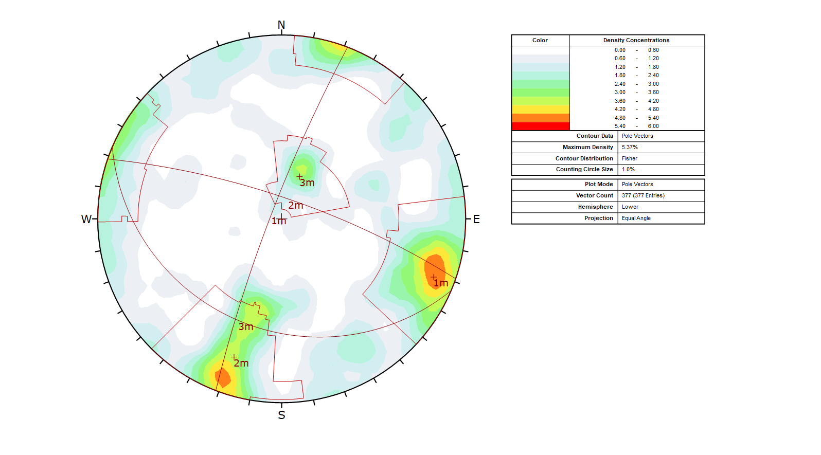
DIPS 2D Stereonet View with 3 joint sets defined - In the Import Synthetic Joints From DIPS dialog:
- Set Terzaghi Weighting = Unweighted. See the Terzaghi Weighting topic from the DIPS User Guide for more
information.
A listing of Joint Sets from the DIPS file is shown with Name, Set ID, the mean Dip and Dip Direction, and Fisher K.RocSlope3 can directly import .dips6, .dips7, and .dips8 files. However, for .dips9 files, only the corresponding .dipsresults file can be used. Refer to the latest DIPS documentation for more information on .dipsresults files. - Select Overwrite Existing Synthetic Joint Properties. This will overwrite the existing
Synthetic Joint Property.
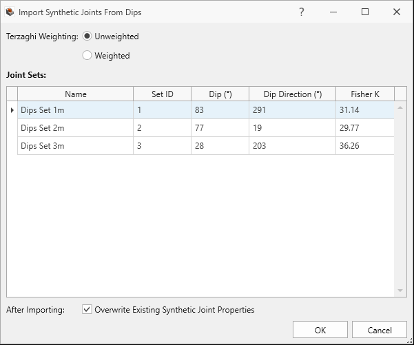
- Click OK to import the three (3) Synthetic Joint Properties from DIPS.
When importing from DIPS, only the Mean Dip, Mean Dip Direction, and Fisher K are imported, used to statistically sample the joint orientations according to the Fisher distribution. See the Fisher Distribution topic from the DIPS User Guide for more information. The Radius and Spacing are set to default values.
Import Synthetic Joints from DIPS dialog - Set Terzaghi Weighting = Unweighted. See the Terzaghi Weighting topic from the DIPS User Guide for more
information.
- For each DIPS Set (1m, 2m, and 3m), edit the
Radius and Spacing Statistics by clicking the
Distribution
 icon to the right of the Mean Radius and
Mean Spacing fields. By default, the Distribution will be set to
None.
icon to the right of the Mean Radius and
Mean Spacing fields. By default, the Distribution will be set to
None.
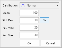
For DIPS Set 1m:- Set Mean Radius = 100, Distribution = Normal
 , Std. Dev. = 10, Rel. Min. = 30. Rel. Max. =
30.
, Std. Dev. = 10, Rel. Min. = 30. Rel. Max. =
30.
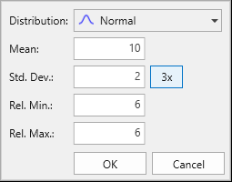
- Set Mean Spacing = 10, Distribution = Normal , Std. Dev. = 2, Rel. Min. = 6, Rel. Max. =
6.
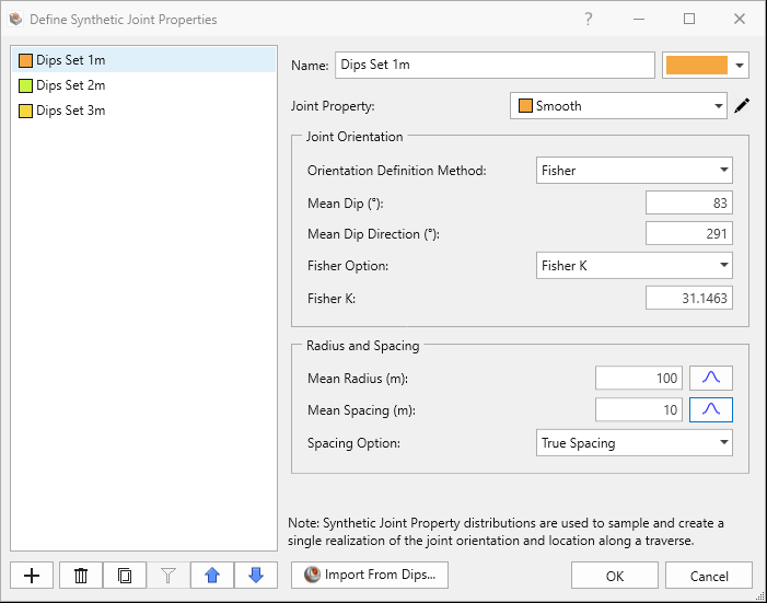
- Set Spacing Option = True Spacing. See the Define Synthetic Joints topic for more
information on Joint Spacing.
Radius Statistics Settings Spacing Statistics Settings DIPS Set 1m Synthetic Joint Property in Define Synthetic Joints dialog - Set Mean Radius = 100, Distribution = Normal
- Repeat Step 5 for DIPS Set 2m and DIPS Set 3m.
- Click OK to save the synthetic joint properties and exit the Define Synthetic Joints dialog.
4.2 Add Synthetic Joint Set
Now define the traverse on which the joint locations are sampled based on the spacing of joints (distribution and spacing option).
To add a synthetic joint set:
- Select Joints > Add Synthetic Joint Set

- Under the Draw Polyline pane, select Edit Table.
- In the Edit Polyline dialog, add 4 rows by clicking the Insert Row
 button at the top of the dialog.
- Specify the X, Y, Z points of the polyline within the rows you created as follows:
| X | Y | Z |
|---|---|---|
| -370 | -517 | 1004 |
| -430 | -388 | 1004 |
| -473 | -228 | 1004 |
| -495 | -92 | 1004 |
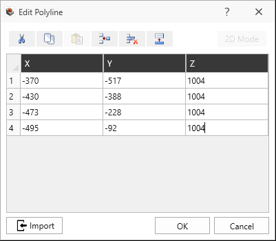
- Click OK.
- Click the Done
 button in the Draw Polyline pane to
finalize the polyline.
button in the Draw Polyline pane to
finalize the polyline. - In the Add Synthetic Joint Set dialog:
- Set Joint Property = DIPS Set 1m.
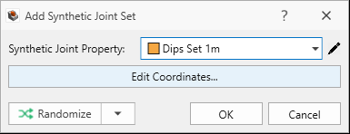
Add Synthetic Joint Set dialog - Click OK to add the synthetic joint set.
- Set Joint Property = DIPS Set 1m.
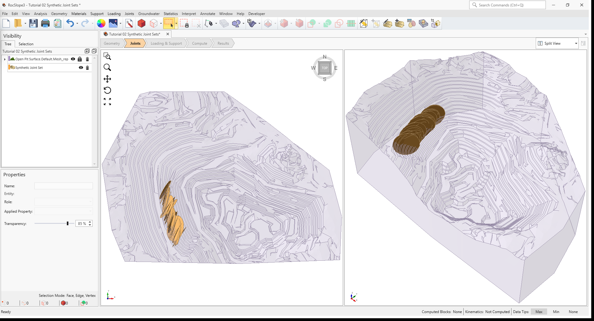
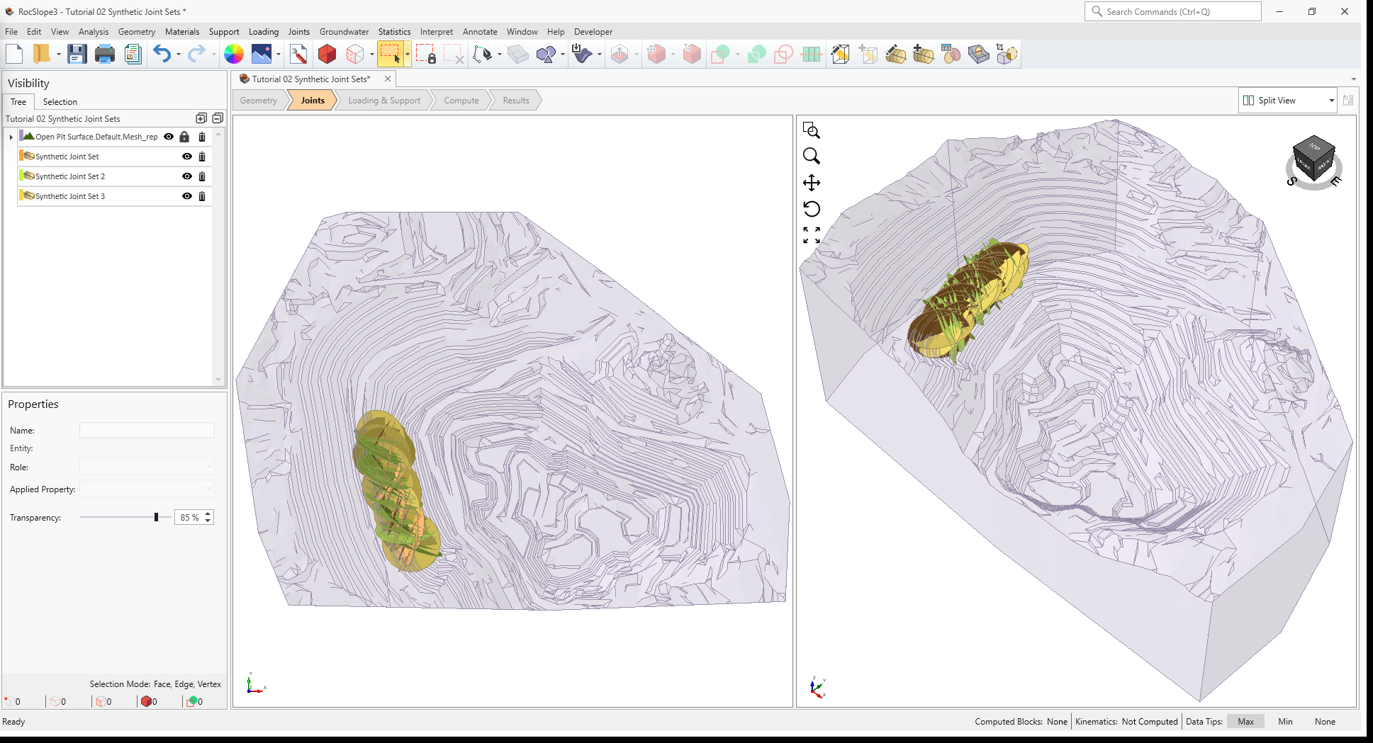
Select the Synthetic Joint Set entity in the Visibility Tree and the entity will be selected (highlighted red). The following information is shown in the Properties pane:
- Name = Synthetic Joint Set
- Applied Property = DIPS Set 1m
- Transparency = 0%, by default
The joints are drawn in the 3D View.
Repeat Steps 1-5 to add the second joint set:
- Select Joints > Add Synthetic Joint Set from the menu or toolbar.
- Under the Draw Polyline pane, select Edit Table.
- In the Edit Polyline dialog:
- Specify the X, Y, Z points of the polyline the same as the first Synthetic Joint Set.
- Click OK.
- Specify the X, Y, Z points of the polyline the same as the first Synthetic Joint Set.
- Click the Done button in the Draw Polyline pane to
finalize the polyline.
- In the Add Synthetic Joint Set dialog:
- Set Joint Property = [DIPS Set 2m].
- Click OK to add the synthetic joint set.
Repeat Steps 1-5 to add the third joint set:
- Select Joints > Add Synthetic Joint Set from the menu or toolbar.
- Under the Draw Polyline pane, select Edit Table.
- In the Edit Polyline dialog:
- Specify the X, Y, Z points of the polyline the same as the first Synthetic Joint Set.
- Click OK.
- Specify the X, Y, Z points of the polyline the same as the first Synthetic Joint Set.
- Click the Done button in the Draw Polyline pane to finalize the polyline.
- In the Add Synthetic Joint Set dialog:
- Set Joint Property = [DIPS Set 3m].
- Click OK to add the synthetic joint set.
The joints are drawn in the 3D View.
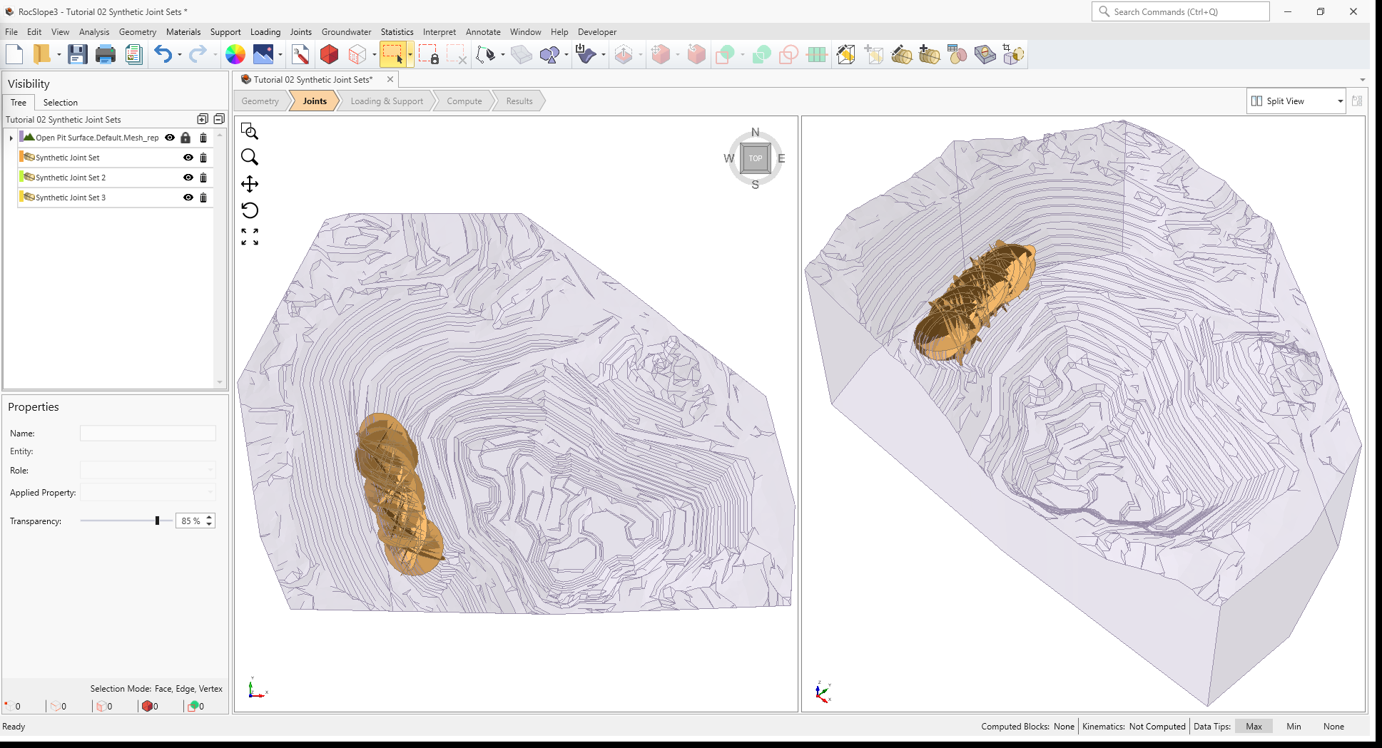
4.3 Joint Colours
By default, all joints are coloured according to the assigned Joint Property colour. In this model
all three Synthetic Joint Sets are assigned the same Joint Property (i.e., Rough) and are therefore it is hard to
distinguish between the sets.
To colour joints by the Synthetic Joint Property:
- Select View > Display Options

- In the Display Options dialog, navigate to the Joints tab.
- Select Use Synthetic Joint Property Color.
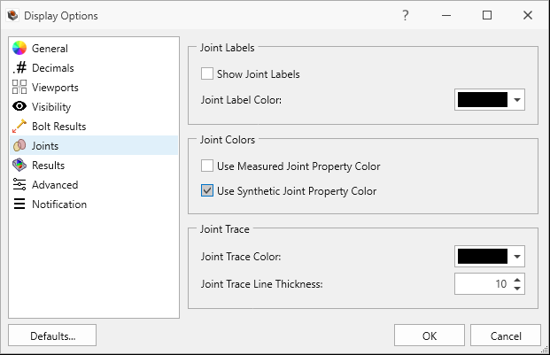
Joints tab in Display Options dialog - Click OK to close the dialog.
The joints are now coloured according to Synthetic Joint Property colours.
4.4 Synthetic Joint Information
To view a listing of all joints belonging to a Synthetic Joint Set:
- Select any of the Synthetic Joint Set nodes from the Visibility Tree.
- Select Synthetic Joint Information button from the Properties pane or select
Joints > View Synthetic Joint Information
 in the menu.
 - The Synthetic Joint Information dialog shows a listing of joints in the set with Dip, Dip
Direction, X, Y, Z, and Radius columns. The information can be copied by clicking the Copy
 button at the bottom-left of the dialog.
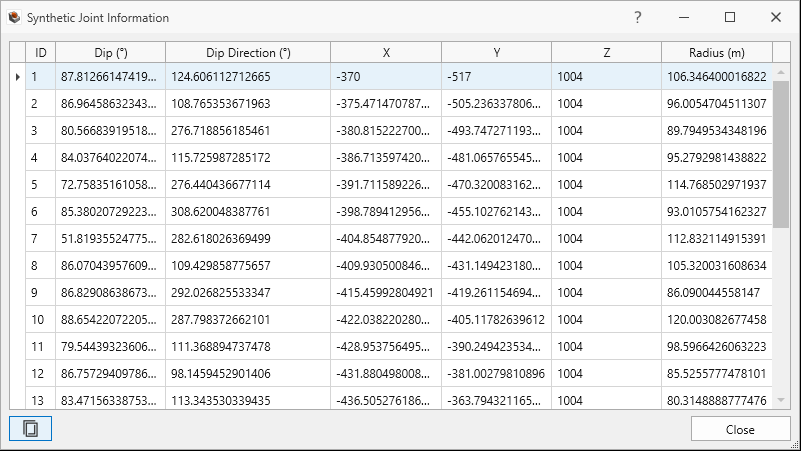
Listing of Joints in Synthetic Joints Information dialog Information in the Synthetic Joint Information dialog is read-only and cannot be modified.
- Click Close to exit the dialog.
4.5 Randomize Synthetic Joint Sets
Synthetic Joint sampling is NOT a probabilistic analysis using joint orientation, radius, and spacing as random variables. We are only sampling the joints in a joint set once to get variations in joint orientation, radius and spacing across the traverse. In other words, the sampling only represents one realization of the joint set. The joint set sampling is determined according to the statistics defined in the applied Synthetic Joint Property (i.e., Orientation, Radius, Spacing), the Traverse polyline, and the Pseudo-random Seed value (default seed = 10116).
The ability to form of blocks, the removability of blocks, and the kinematics of blocks are extremely dependent on the joint's orientation, persistence, and spatial location. In some cases, a user may want to see different realizations of the Synthetic Joint Sets so that a different statistical sampling of the synthetic joints are generated and potentially a different collection of blocks.
To regenerate the sampling for a Synthetic Joint Set:
- Select any of the Synthetic Joint Set nodes from the Visibility Tree.
- Under the Properties pane, select Edit to edit the geometry.
- In the Edit Synthetic Joint Set dialog:
- Click the Randomize
 button to randomly pick a new
Pseudo-random Seed value. Note that the joints in Synthetic Joint Set 1
have been sampled again using the same distributions but different randomization.
button to randomly pick a new
Pseudo-random Seed value. Note that the joints in Synthetic Joint Set 1
have been sampled again using the same distributions but different randomization. 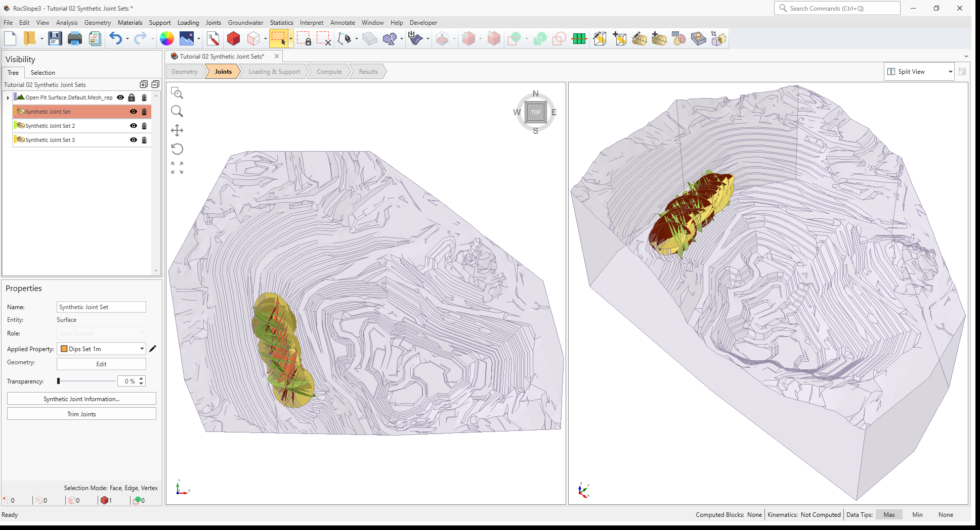
Randomized realization of the Synthetic Joint Set may not appear as displayed for user model - Repeatedly click the Randomize button a few times to get different realizations.
- Select the dropdown from the Randomize button and select Edit Random
Seed
 .The Random Seed dialog shows the current
Pseudo-random Seed value.
.The Random Seed dialog shows the current
Pseudo-random Seed value. - Select the dropdown from the Randomize button and select Reset Random
Seed. The Pseudo-random Seed value is reset back to the default seed value
of 10116. Joint Set 1 will be sampled identically to the initial realization of the
joints.
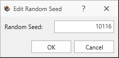
Edit Random Seed Dialog showing default seed value - Click OK to close the Edit Synthetic Joint Set dialog.
- Click the Randomize
5.0 Compute
RocSlope3 has a two-part compute process.
5.1 Compute Blocks
The first step is to compute the unit blocks which may potentially be formed by the intersection of joints with other joints and the intersection of joints with the free surface.
To compute the unit blocks:
- Navigate to the Compute workflow tab

- Select Analysis > Compute Blocks

As compute is run, the progress bar reports the compute status. Once compute is finished, the Results
node is added to the Visibility Tree and All Valid Unit Blocks are blocks are
shown in the 3D View. The Results node consists of the collection of valid unit blocks and the
socketed slope. The original External and Synthetic Joint Set(s) visibility is turned off.
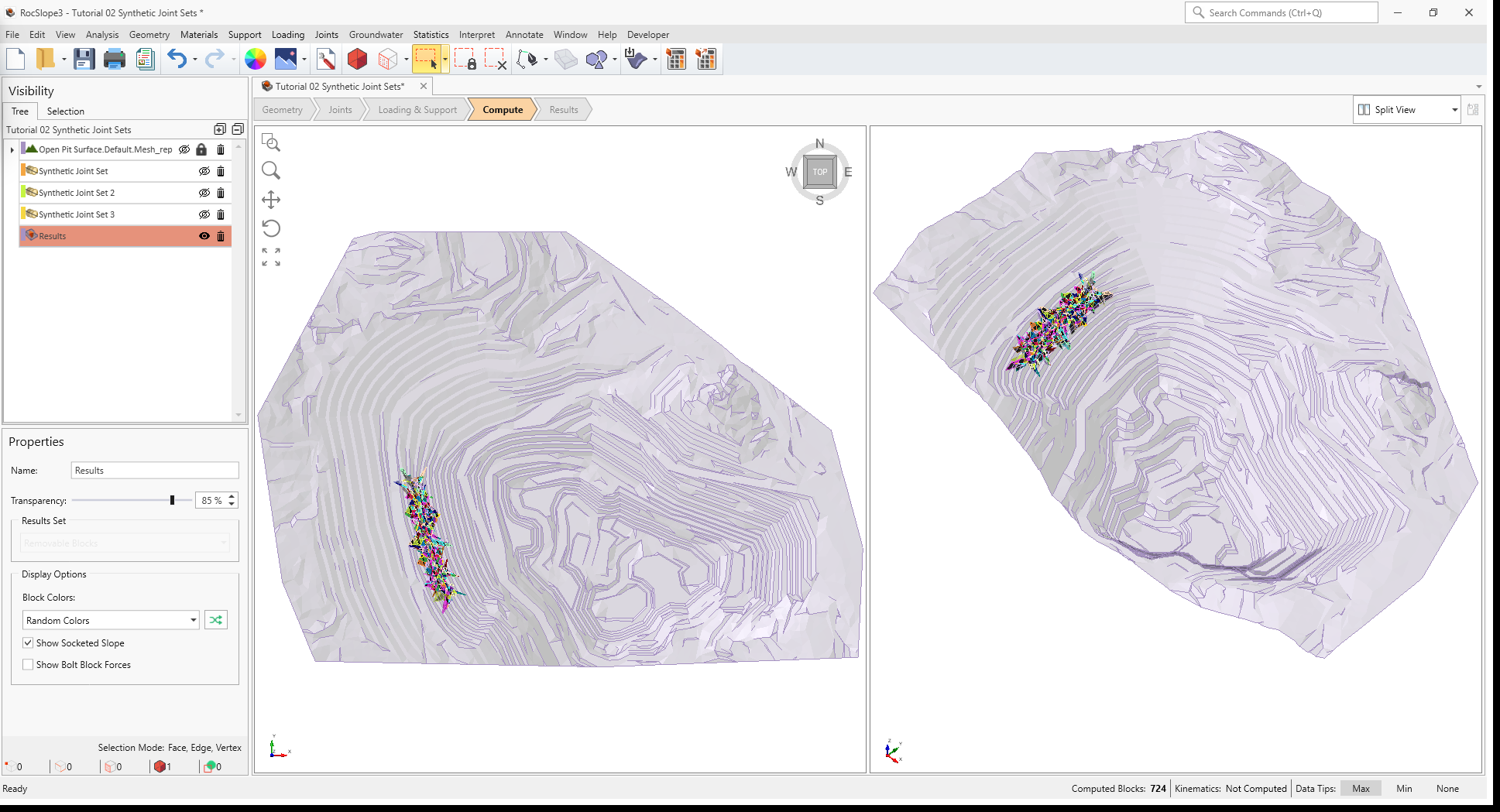
Once compute is finished, the unit blocks are coloured according to the Block Color option (Random Colors) set in the Results node's Property pane.
Compute Blocks only determines the geometry of the unit blocks. In order to obtain other information such as the factor of safety, Compute Kinematics needs to be run.
5.2 Compute Kinematics
The second and final compute step is to compute the removability, forces, and factor of safety for each of the valid unit blocks.
To compute the block kinematics:
- Ensure that the Compute workflow tab is the active workflow.
- Select Analysis > Compute Kinematics

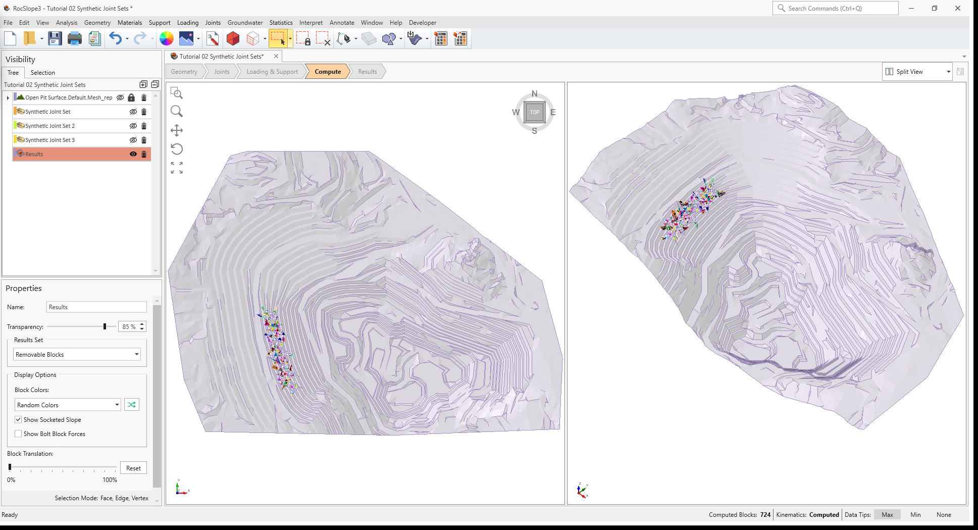
As compute is run, the progress bar reports the compute status. By default, after Compute Kinematics
is run, only Removable Unit Blocks are shown.
6.0 Interpreting Results
Once both blocks and kinematics are computed, all block results can be viewed in a table format.
6.1 Block Information
To view all block results:
- Navigate to the Results workflow tab

- Make sure that Block Type = Unit Blocks and Results Set = Removable Unit Blocks in the Results node Properties pane.
- Select Interpret > Block Information

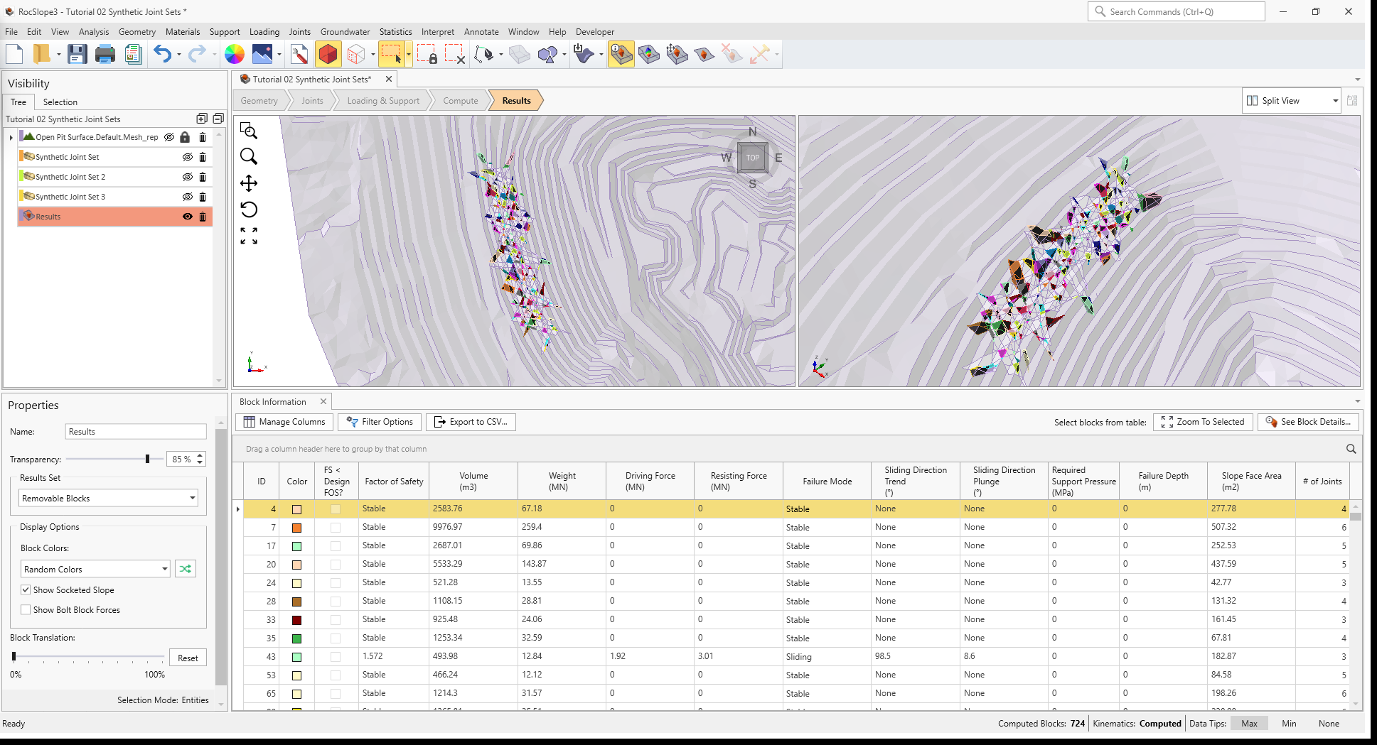
The Block Information pane shows the collection of blocks according to the Block Type and Results Set
settings. The Block Type and Results Set shown can be selected in the Results tab of the Display Options, or the Properties pane for the Results Node. In this case, only Removable Unit Blocks are
coloured and listed in Block Information.
Visualizing blocks can be difficult when the slope extents are large compared to the block extents.
To zoom to a selected block:
- Select a row (or multiple rows by holding CTRL) in the Block Information listing.
- Select Zoom to Selected
 above the Block Information listing (or Zoom to Selected Blocks
  in the Interpret menu).
To zoom into all blocks:
- Select Interpret > Zoom To All Blocks

6.2 Contour Blocks
Not only are the magnitudes of critical values such as the block's factor of safety or weight important to be aware of, the location also matters. The Contour Blocks option allows the user to plot a safety map of various block metrics so that the range of values can be visualized over the slope. Let's show the contour of Factor of Safety for only Failed Unit Blocks.
To show block contours for failed blocks:
- Select the Results node from the Visibility Tree.
- In the Results node Properties pane, set Block Type = Unit Blocks and Results Set = Failed Unit Blocks (FS < Design FS).
- Select Interpret > Contour Blocks

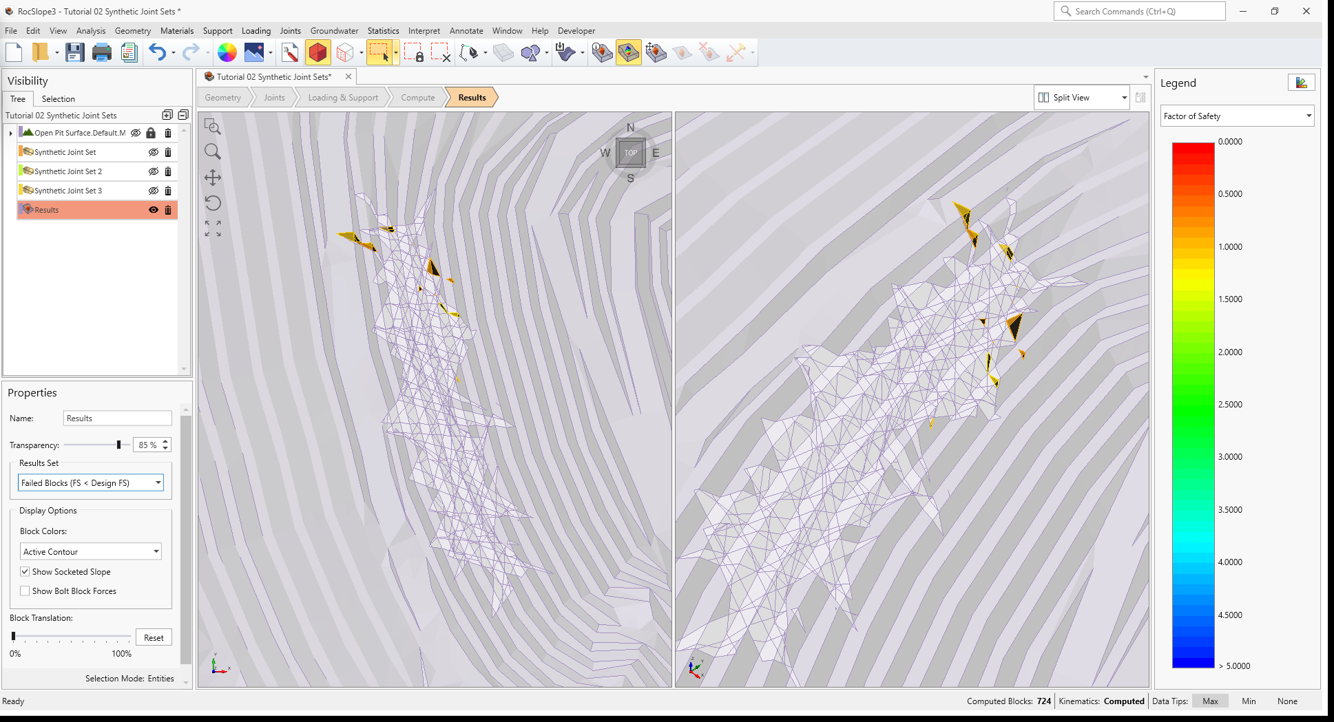
- From the Legend pane to the right, select Factor of Safety from the dropdown.
All the failed unit blocks are contoured by Factor of Safety. The minimum Factor of Safety blocks are contoured RED while the blocks with Factor of Safety > 5 are contoured BLUE.
This concludes Tutorial 02.