1 - Quick Start
1.0 Introduction
This tutorial introduces some of the basic features of RocSlope3. The model used in this tutorial is an open pit with measured structures (i.e., joints) of known orientation, size, and location. Assuming that the failure of the slope is structurally-controlled, we will be using the defined joint surfaces to form blocks which may become unstable.
Finished Product
The finished product of this tutorial can be found in the Tutorial 01 Quick Start folder. All tutorial files installed with RocSlope3 can be accessed by selecting File > Recent Folders > Tutorials Folder from the RocSlope3 main menu.
2.0 Starting a Model
Open RocSlope3. You will see a blank workspace.
2.1 Project Settings
Our first step is to configure the analysis parameters for the model in Project Settings.
- Select Analysis > Project Settings or click on the Project Settings
 icon in the toolbar.
 - Select the Units tab.
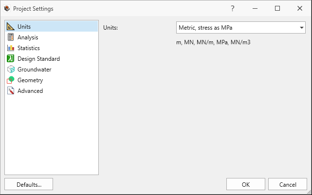
Units Tab in Project Settings Dialog - Set Units to Metric, stress as MPa and keep everything else as default.
- Select the Analysis tab.RocSlope3 has two types of blocks:
- Unit blocks are individual blocks that form from the intersection of joints and the slope surface.
- Combined blocks are combinations of unit blocks that represent the largest removable block. See the Analysis topic for more information.
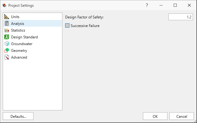
Analysis Tab in Project Settings Dialog - Set Design Factor of Safety = 1.2.
- Set Successive Failure = OFF. We will only be analyzing the blocks which daylight and are readily removable.
- Set Combined block (computes largest removable) = OFF. We will only be analyzing unit blocks in this tutorial.
- Click OK to save the settings and close the dialog.
3.0 Defining Material Properties
RocSlope3 is designed with an intuitive workflow to help guide the user through the required steps in creating a model. Under each workflow tab, the toolbars and menus are customized to provide the user with the functions needed in each step of creating the model.
We will begin with the Geometry workflow tab to define the materials.
- Navigate to the Geometry workflow tab

- Select Materials > Define Materials in the menu or click the Define Materials
 icon in the toolbar.
The Define Materials dialog allows users to define the Unit Weight of the rock and Groundwater Settings.
Since the failure is assumed to be structurally-controlled, rock mass strength is not considered in a RocSlope3 analysis; instead, the shear strength of the joints (defined in the Define Joint Properties dialog) are used to model shear resistance to sliding. - Select Material 1 from the list on the left side of the dialog. Enter the following properties
for Material 1.
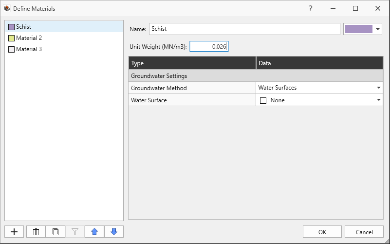
Schist Material Property in Define Materials Dialog - Name = Schist
- Unit Weight = 0.026 MN/m3
- Leave the default Groundwater Settings (i.e., no groundwater applied).
- Select Material 2 from the list on the left side of the dialog.
- Click the Delete
 button on the bottom-left of the dialog to
delete Material 2.
button on the bottom-left of the dialog to
delete Material 2. - Repeat these same steps to delete Material 3.
- Click OK to save the changes and close the Define Materials dialog.
4.0 Creating Geometry
We will be using a pit shell surface geometry to create the external geology.
4.1 Import Geometry
To import the pit shell surface geometry into RocSlope3:
- Ensure the Geometry workflow tab is still active.
- Select File > Import > Import Geometry
 . Several geometry file formats are supported. See the Import Geometry topic for more information.
 - In the Open dialog, select the Open Pit Surface.rsgeomobj file in the Tutorial 01 Quick Start folder (located in your installation folder) and click Open.
The Import Geometry dialog shows the file and mesh entities available for import and a preview of the entity. - Ensure Geometry Role = Geology in the drop down at the top-left of the Import Geometry dialog.
- Select the All Geometry checkbox to select all the entities (in this case, only one
'Mesh' entity exists).
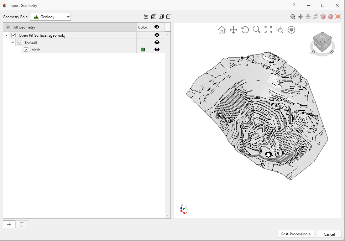
Open Pit Surface geometry preview in Import Geomoetry Dialog - Click the Post-Processing button in the bottom-right of the dialog.
- Click Done to import the geometry.
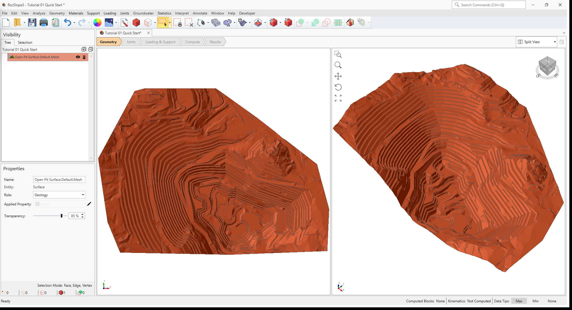
The geometry is imported into RocSlope3 and added to the Visibility Tree. The Visibility pane is located on the top-left of the application window and shows a tree of entity objects in the model.
Click the Open Pit Surface.Default.Mesh entity in the Visibility Tree. The entity will be selected (highlighted red) and the following information is shown in the Properties pane (below the Visibility pane):
- Name = Open Pit Surface.Default.Mesh
- Entity = Surface
- Role = Geology
- Transparency = 85%, by default
4.2 Create External Volume from Surface
To create a valid external for modelling, we have to convert the surface of the open pit to a volume.
To create the external volume from a surface:
- Select the Open Pit Surface.Default.Mesh surface from the Visibility Tree. The entity is highlighted in the 3D View.
- Select Geometry > Create External From Surface

The Create External From Surface dialog allows the user to set the bottom of the volume (either by Elevation or by Depth).
- In the Elevation tab, set the Bottom Elevation = 500.
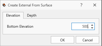
Create External from Surface Dialog - Click OK to extrude the model down to an elevation of 500 m and set the volume as an External.
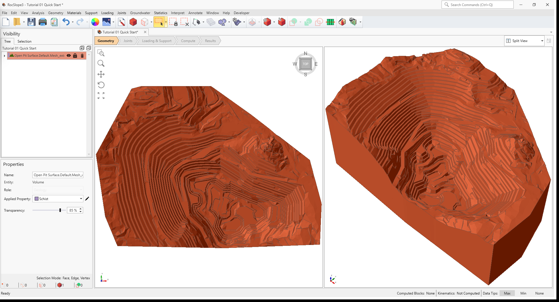
Select the Open Pit Surface.Default.Mesh_extruded entity in the Visibility Tree. The entity will be selected (highlighted red), and the following information is shown in the Properties pane:
- Name = Open Pit Surface.Default.Mesh_extruded
- Entity = Volume
- Role = Geology
- Applied Property = Schist
- Transparency = 85%, by default
- The Block's weight since the total weight of the block is the sum of all volume pieces and each piece may have a different Unit Weight (from Define Material Properties dialog).
- The Joint's shear strength if the Strength is set to Override by Material. See the Shear Strength topic for more information.
- The Joint's water pressure if the Water Pressure Method is set to Material Dependent. See the Joint Water Pressure topic for more information.
In this model, there is only one (1) Material Volume assigned with the Schist material property.
5.0 Defining Joint Properties
Without the consideration of loads and supports (i.e., self-weight of blocks only), the stability of a geometrically removable block depends on the shear strength of the joints on which it slides.
To define joint properties:
- Navigate to the Joints workflow tab

- Select Joints > Define Joint Properties or click on the Define Joint Properties
 icon in the toolbar.
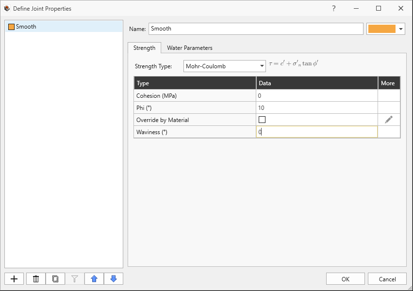
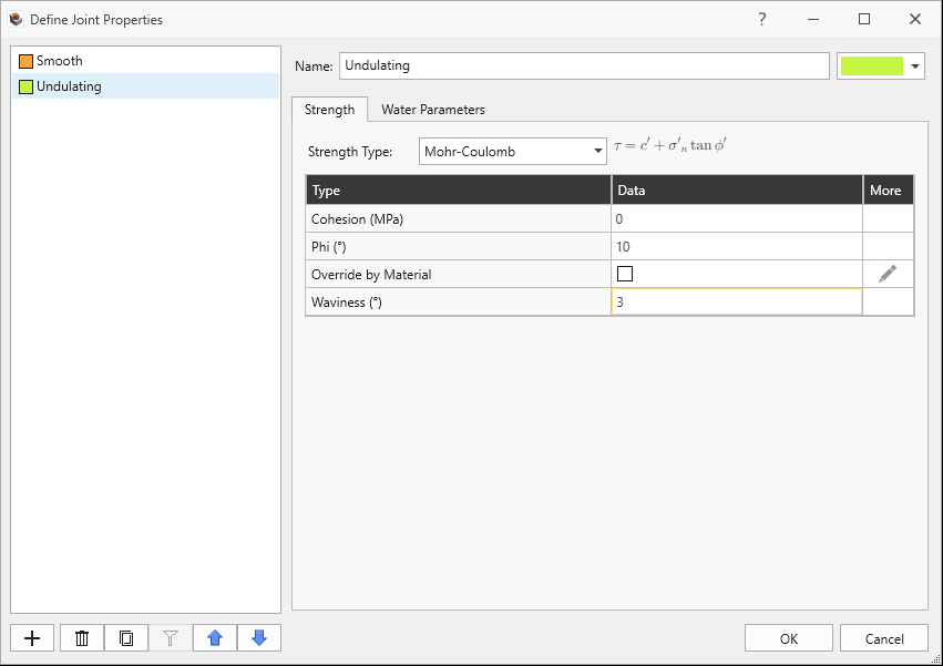
The Define Joint Properties dialog allows users to define the Strength Model, Waviness, and Water Pressure for each joint property.
- Select Joint Property 1 from the list on the left side of the dialog. Enter the following properties for Joint Property 1:
- Name = Smooth
- Under the Strength tab:
- Strength Type = Mohr-Coulomb
- Cohesion = 0 MPa
- Phi = 10 deg
- Override by Material = OFF
- Waviness = 0 deg
- Water Pressure Method = Dry
 button below the list of materials, at the
bottom-left of the dialog. Enter the following properties for Joint Property 2:
button below the list of materials, at the
bottom-left of the dialog. Enter the following properties for Joint Property 2:- Name = Undulating
- Under the Strength tab:
- Strength Model = Mohr-Coulomb
- Cohesion = 0 kPa
- Phi = 10 deg
- Override by Material = OFF
- Waviness = 3 deg
- Water Pressure Method = Dry
The two joint properties model joints which are heavily weathered, providing very little shear resistance.
6.0 Adding Measured Joints
In this example, we will be defining the joints using measured orientation data from a CSV file. We can easily add a list of joints where for each joint, the orientation, location and size is known.
To define measured joints:
- Ensure the Joints workflow tab is still active.
- Select Joints > Define Measured Joints or click on the Define Measured Joints
 icon in the toolbar.
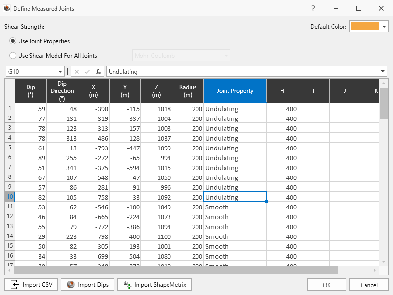
The Define Measured Joints dialog is an Excel-like spreadsheet which allows users to easily input, drag, copy, paste, and import data. Formulas are also supported. Each row represents a single joint. Each joint is defined by a Dip, Dip Direction, and modeled as a planar disk with its center at Location X, Y, Z, and a Radius. A different Joint Property can be assigned to each joint using either the Joint Properties defined in Define Joint Properties dialog, or by specifying a different set of shear parameters for a given Shear Model.
- Select Use Joint Properties. We will be assigning the Joint Property from one
of the two joint properties defined from earlier.
For this demonstration, we will be importing the orientation data directly from a CSV file.
- Click Import CSV

- In the Open dialog, select the Upper West Joint Mapping Data.csv file from the Tutorials 01 Quick Start folder and click Open.
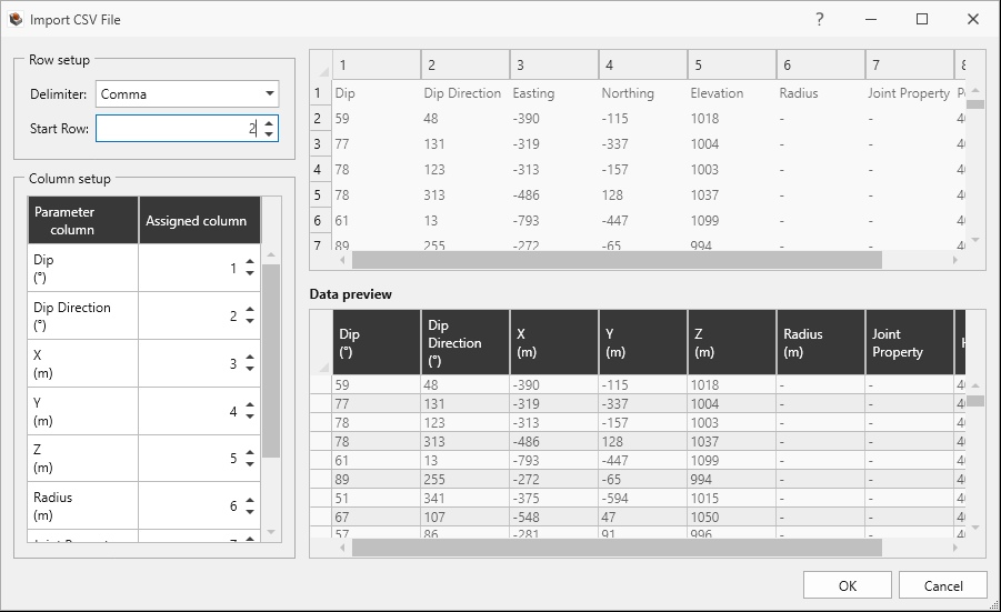
- In the Import CSV File dialog:
- Set the Data Delimiter = Comma.
- Set the Start Row = 2 to skip the first header row.
- Under the Data Column Selection, set the following indices:
- Dip = 1
- Dip Direction = 2
- Location X = 3
- Location Y = 4
- Location Z = 5
- Radius = 6
- Joint Property = 7
- Additional column H = 8
Formulas in this grid control work like Microsoft Excel formulas, which is denoted by "=" followed by an expression. There are also various built in functions which have the same notation as Microsoft Excel.
- Right-click and select Assign Joint Property to All > Smooth. All populated rows are assigned with Smooth under the Joint Property column.
- Select the cells in the Joint Property column from Rows 1 through 10. Right-click and select Assign Joint Property to Selected > Undulating. The selected (10) rows are assigned with Undulating (as shown below).
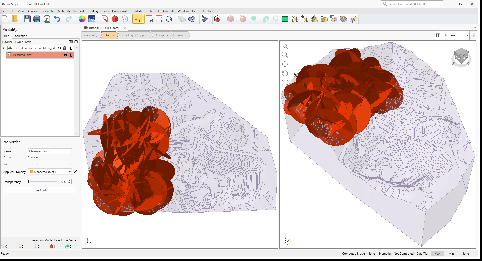
Select the Measured Joints entity in the Visibility Tree. The entity will be selected (highlighted red) and the following information is shown in the Properties pane:
- Name = Measured Joints
- Applied Property = Measured Joint 1 (currently, only one set of Measured Joint data is supported by RocSlope3)
- Transparency = 0%, by default
The joints are drawn in the 3D View.
7.0 Compute
RocSlope3 has a two-part Compute process.
7.1 Compute Blocks
The first step is to compute the unit blocks which may potentially be formed by the intersection of joints with other joints and the intersection of joints with the free surface.
To compute the unit blocks:
- Navigate to the Compute workflow tab

- Select Analysis > Compute Blocks or click the Compute Blocks
 icon in the toolbar.
As compute is run, the progress bar reports the compute status. Once compute is finished, the Results
node is added to the Visibility Tree and All Valid Unit Blocks are shown in
the 3D View. The Results node consists of the collection of valid unit blocks and the socketed
slope. The original External and Measured Joints visibility is turned off.
The unit blocks are coloured according to the Block Colors option. The Block Colors settings can be edited in the Results node's Property pane or in the Display Options dialog. By default, Block Colors is set to Random Colors, which colours each adjacent block a different colour to be able to easily distinguish between different blocks. The program's default Block Colors can be changed in the Display Options dialog.
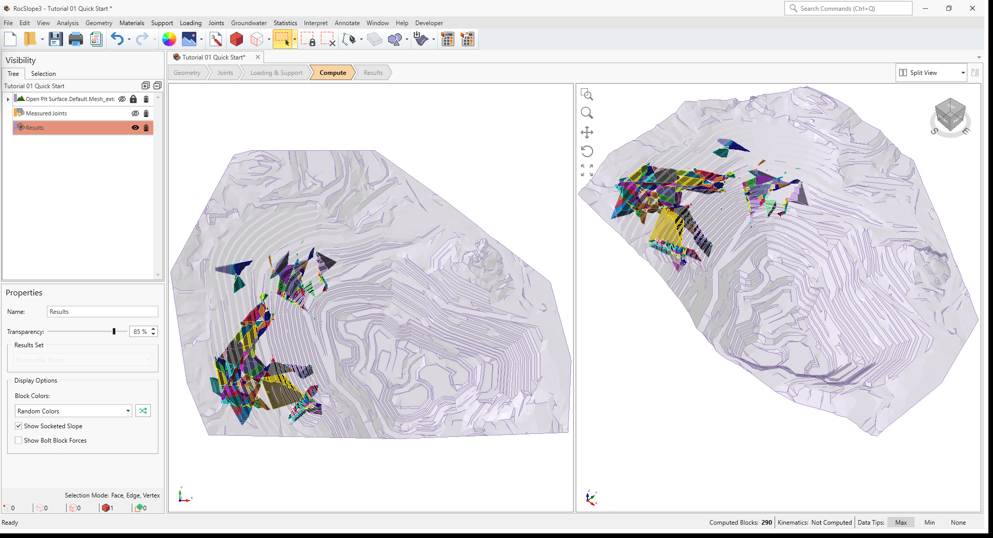
For this tutorial, 290 unit blocks have been computed (some may be invalid). This is indicated by the "Unit: 290" on the status bar at the bottom-right of the application window. This status bar also indicates what Result Type is shown in the viewport (Unit Blocks, Combined Blocks, or Unit and Combined Blocks). The Result Type for this model should show Unit Blocks.
Compute Blocks only determines the geometry of the unit blocks. In order to obtain other information such as the factor of safety, Compute Kinematics needs to be run.
7.2 Compute Kinematics
The second and final compute step is to compute the kinematics for each of the valid blocks, including the removability, forces, and factor of safety.
To compute the block kinematics:
- Ensure that the Compute workflow tab is selected.
- Select Analysis > Compute Kinematics or click on the Compute Kinematics
 option in the toolbar.
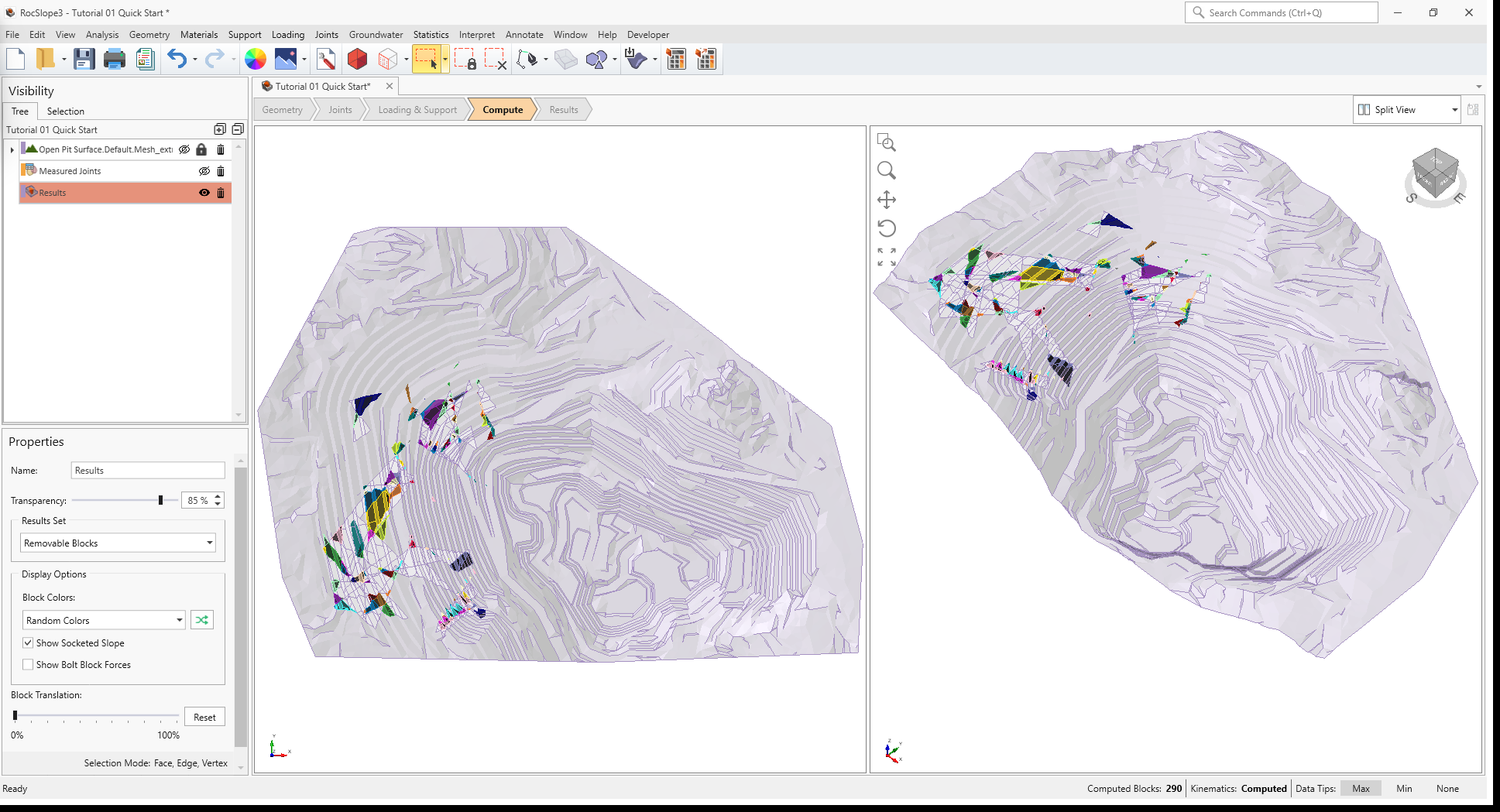
As compute is run, the progress bar reports the compute status. By default, after Compute Kinematics
is run, only Removable Unit Blocks are shown.
To show all blocks:
- Select View > Display Options or click on the Display Options
 icon in the toolbar.
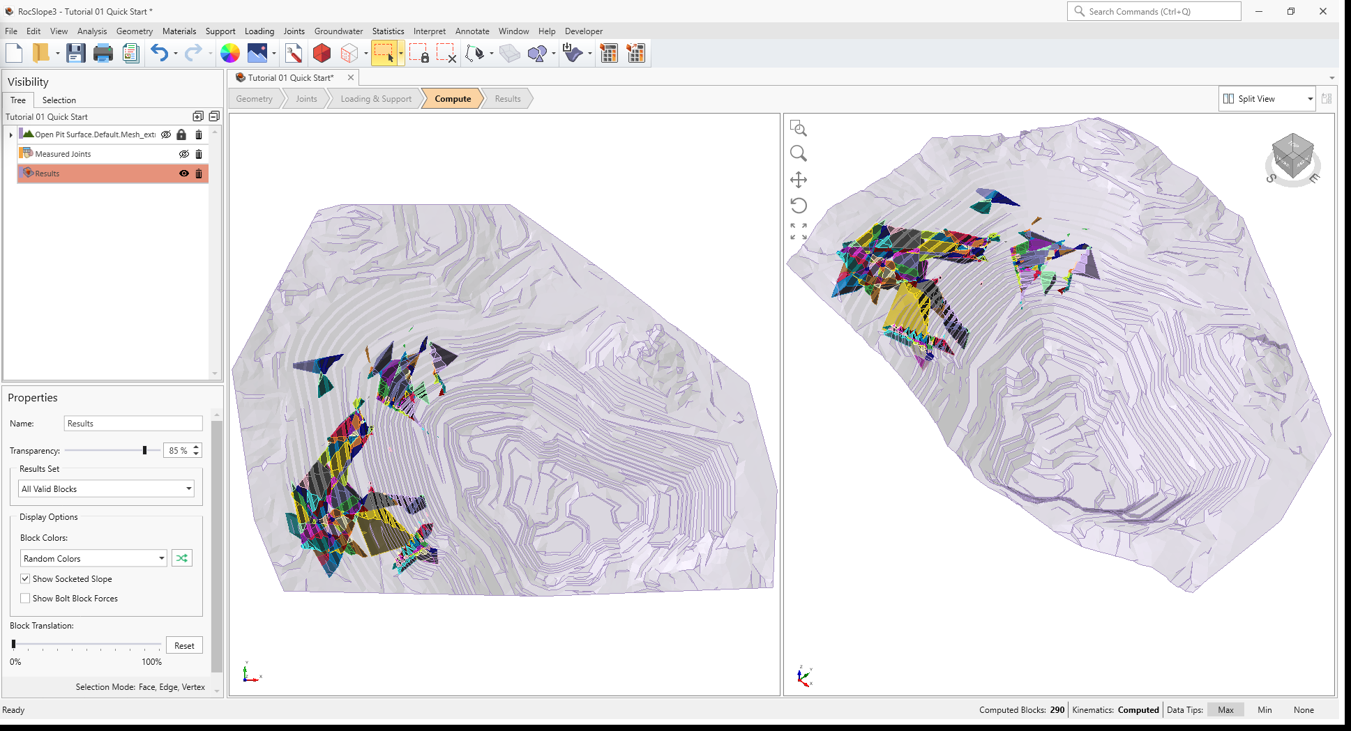
 - In the Display Options dialog:
- Navigate to the Results tab
- Set Block Type = Unit Blocks
- Set Results Set = All Valid Unit Blocks
- Click OK to close the dialog.
Alternatively, the Results Set can also be selected from the Properties pane of the Results node. Removable Unit Blocks, Removable Combined Blocks, Failed Unit Blocks (FS < Design FS), and Failed Combined Blocks (FS < Design FS) Results Set options are only available once Compute Kinematics is run.
The status of the kinematic compute is indicated by the "Kinematics: Computed" on the status bar at the
bottom-right of the application window.
8.0 Interpreting Results
Once both blocks and kinematics are computed, all block results can be viewed in a table format.
8.1 Block Information
To view all block results:
- Navigate to the Results workflow tab

- Make sure that Block Type = Unit Blocks and Results Set = All Valid Unit Blocks in the Results node Properties pane.
- Select Interpret > Block Information or click on the Block Information
 option in the toolbar.
Visualizing blocks can be difficult when the slope extents are large compared to the block extents.
To zoom into all blocks:
- Select Interpret > Zoom To All Blocks

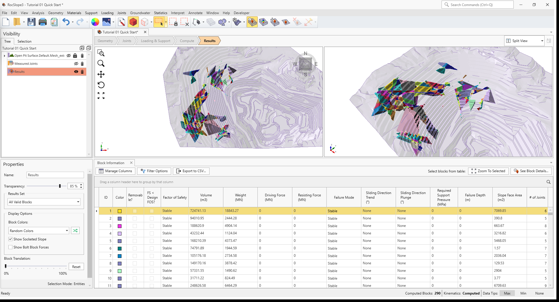
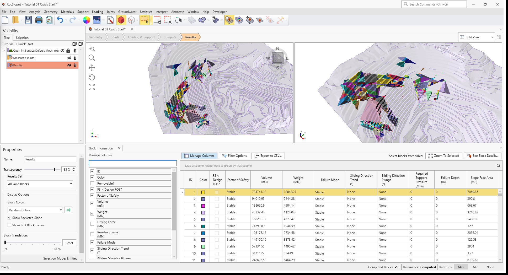
The Block Information pane shows the collection of blocks according to the Block Type and Results Set settings. The Block Type and Results Set shown can be selected in the Results tab of the Display Options, or the Properties pane for the Results Node. Currently, All Valid Unit Blocks are listed.
A number of columns are available including:
- ID
- Color (colour which corresponds to the block's colour in the 3D View)
- Removable?
- FS < Design FOS?
- Factor of Safety
- Volume
- Weight
- Driving Force
- Resisting Force
- Failure Mode
- Sliding Direction Trend
- Sliding Direction Plunge
- Required Support Pressure
- Slope Face Area
- # of Joints
Any of the columns can be hidden. Let's hide the Volume, Driving Force, Resisting Force, and the # of Joints columns.
- Click on Manage Columns
 on the left side of the Block Information pane.
 - Uncheck Volume, Driving Force, Resisting Force, and # of Joints.
The columns are now hidden.
The rows of block data can also be filtered. Let's filter by blocks which have a Weight >= 10 MN.
- Click Filter Options

- Click the arrow to expand the Edit Filters section on the left side of the Block Information pane.
- Set the Weight minimum = 10 (MN).
- Hit ENTER.
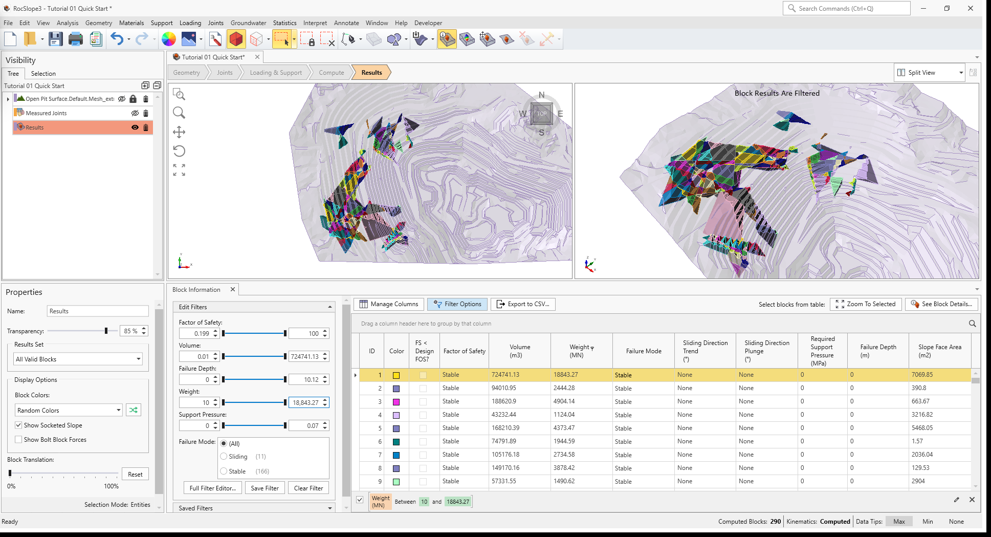
Blocks which are filtered out are not listed in the Block Information table and are also not colored according to the Block Colors option (e.g., Random Colors, Active Contour) selected in the 3D View. A message "Block Results are Filtered" is displayed at the top center of the Perspective Viewport. More advanced filtering criteria can be specified in the Full Filter Editor. See the Filter topic for more information.
To save the current filter:
- Click the Save Filter button at the bottom of the Edit Filters section.
- In the Save Filter dialog:
- Select Save As New Filter.
- Enter the name of the filter.
- Click OK to save the filter and close the dialog.
A list of saved filters can be selected from at a later time under the Saved Filters section from the left of the Block Information pane.
To remove the current filter:
- Select the Clear Filter button at the bottom of the Edit Filters pane.
To see the detailed information for a given block:
- Select the Block ID. For this example, we will select Block ID = 32 from the rows of the Block Information (or graphically, by clicking the Block in the 3D View).
- Click the See Block Details
 button at the top of the Block Information pane.
The Detailed Block Information dialog for Unit Blocks shows the 3D model of the Block, general block information as well as detailed information for Joints, Joint Line of Intersection, and Block Vertices.
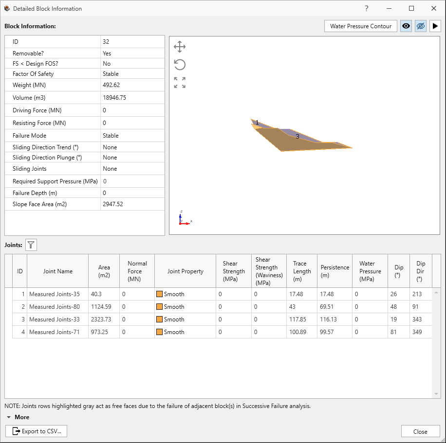
Detailed Block Information Dialog for Block ID = 32 - Select the Filter
 button at the top of the Joints table to modify the
visibility of columns in the table.
button at the top of the Joints table to modify the
visibility of columns in the table. - Check or uncheck any column headers to show or hide columns in the Column Chooser dialog.
- Click the X button to close the Column Chooser dialog.
- Click on the More/Less control at the bottom-left of the Detailed Block Information dialog, to expand or collapse the section containing the Joint Line of Intersections and Blocks Vertices tables.
- Export the block information to CSV using the Export to CSV
 button at the bottom-left of the
Detailed Block Information dialog.
button at the bottom-left of the
Detailed Block Information dialog. - Click Close to exit the dialog.
8.2 Contour Blocks
Not only are the magnitudes of critical values (such as the block's factor of safety or weight) important to be aware
of, the location also matters. The Contour Blocks option allows the user to plot a safety map of
various block metrics so that the range of values can be visualized over the slope.
To show block contours:
- Select Interpret > Contour Blocks or click on the Contour Blocks
 option available in the toolbar.
 - From the Legend pane to the right, select Factor of Safety from the second drop down.
All the removable unit blocks are coloured according to the Factor of Safety contour legend. The minimum Factor of Safety blocks are
contoured RED while the blocks with Factor of Safety > 5 are contoured BLUE. The Contour Options  can be customized.
See the Contour Options topic for more information.
can be customized.
See the Contour Options topic for more information.
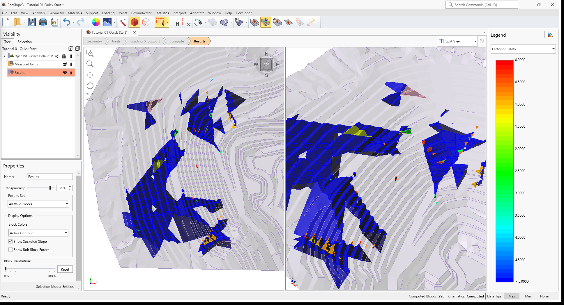
From this heat map of Factor of Safety, locations with the lowest factors of safety and highest failure risk can be identified.
To contour unit blocks by failed weight:
- In the Visibility Tree, select the Results node.
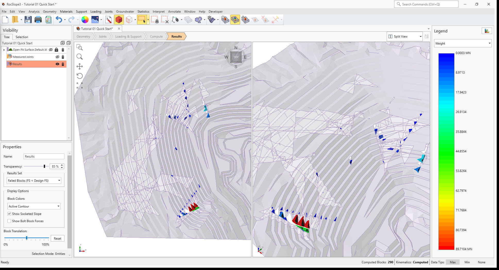
- In the Properties pane, use the drop down to set Block Type = Unit Blocks and Results Set = Failed Unit Blocks (FS < Design FS).
- In the Legend pane to the right, select Weight from the second drop down.

From this heat map of failed unit block weight, locations with the largest failed volumes can be identified.
8.3 Translate Blocks
Translation animation of the blocks is possible for any blocks (unit or combined) which are Removable (i.e., can be removed in at least one valid direction out of the joint socket). For the current Results Set = Failed Unit Blocks (FS < Design FS), all unit blocks are removable since failed blocks are essentially a subset of removable blocks (i.e., a block that is not removable cannot possibly fail).
To translate a block:
- Select Interpret > Translate Blocks
 (or right-click and select Translation >
Translate Blocks).
(or right-click and select Translation >
Translate Blocks). - Select a block graphically by left-clicking, holding and dragging a block in the 3D View.
- When done, right-click and select Done to exit the block translation mode.
To translate all blocks:
- Select the Results node from the Visibility Tree.
- In the Properties pane, use the Block Translation slider to translate all blocks.
To reset the block translation:
- Select Interpret > Reset Translation > Reset Selected Blocks
 or Reset All Blocks
  to move the blocks back into the socket; OR
- Click the Reset button from the Results node's Property pane, beside the Block Translation slider.
This concludes Tutorial 01.