7 - ShapeMetriX Integration
1.0 Introduction
This tutorial demonstrates RocFall3’s ShapeMetriX Geometry Import option. It also demonstrates how the integration and interoperability of ShapeMetriX and RocFall3 streamlines the 3D rockfall analysis workflow, from data acquisition in the field. The tutorial will help you become familiar with importing ShapeMetriX 3D Models to generate a RocFall3 model, and perform a 3D rockfall analysis in RocFall3.
Topics Covered in this Tutorial:
- Importing 3D Model from ShapeMetriX
- Results Interpretation
Finished Product:
The finished product of this tutorial can be found in the Tutorial 07 ShapeMetriX Integration folder, located in the Examples > Tutorials folder in your RocFall3 installation folder.
2.0 ShapeMetriX 3D Model Generation
ShapeMetriX is a comprehensive software suite designed for geologic mapping and geometric analysis, equipped with an advanced 3D model generator. It is ideal for creating 3D models of rock surfaces, rock slopes, tunnel faces and walls, etc. using digital imagery or by importing 3D datasets (E57 laser scanner or OBJ data) and performing fast, detailed, non-contact geological mapping and geometric assessment.
MultiPhoto, the first main component of ShapeMetriX, uses multiple overlapping images from standard drones and handheld cameras, including smartphones as input and generates 3D models by estimating the 3D structure of a scene from a set of 2D images using the Structure from Motion (SfM) process. Additionally, MultiPhoto includes standard and constrained referencing features that reference the 3D model to a higher-level coordinate system using externally surveyed Ground Control Points (GCP).
3D Model Generation and Referencing are discussed in more detail in ShapeMetriX Tutorial 1 – 3D Model Generation and Tutorial 2 – Standard and Constrained Referencing Using Ground Control Points.
3.0 3D Model
The model used in this tutorial is a 15m high and approximately 90m long bench face from an open pit mine. The 3D model is generated in ShapeMetriX’s MultiPhoto tool using 72 aerial images.
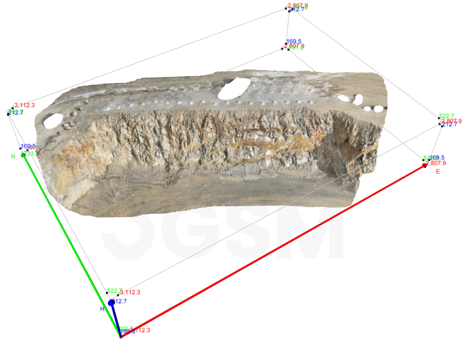
The 3D model geometry is exported as a RocFall3 readable file (.3grs). This exported file will be used as the input file in RocFall3 and can be found in the Examples > Tutorials folder in your RocFall3 installation folder.
3.1 Project Settings
- Select Analysis > Project Settings

- In the Units tab, ensure that Units is set to Metric.
In the Methods tab, ensure that the Analysis Type is set to Lump Mass and that Consider Rotational Velocity is selected.
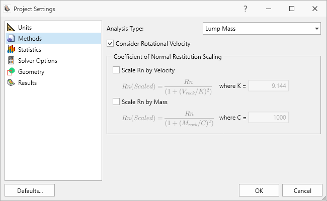
Methods tab in Project Settings dialog - Click OK.
3.2 Material Properties
- Select Materials > Define Materials
 . This opens up the Define Material Properties dialog.
 - The program has 3 built-in materials. We will only be using the first material (Bedrock Outcrops) in this tutorial. We will use the default values for the Normal Restitution, Tangential Restitution, and Friction Angle.
- Delete
 the other two materials (Talus Cover, Asphalt) in the Define Material Properties dialog.
The Define Materials Properties dialog should only have one material (Bedrock Outcrops). The Bedrock Outcrops material property values should look as follows when the All Statistics ![]() button is clicked:
button is clicked:
| Property | Distribution | Mean | Std. Dev. | Rel. Min. | Rel. Max. |
| Normal Restitution | Normal | 0.35 | 0.04 | 0.12 | 0.12 |
| Tangential Restitution | Normal | 0.85 | 0.04 | 0.12 | 0.12 |
| Friction Angle | None | 30 | - | - | - |
3.3 Import Geometry
To import the Bench Face geometry into RocFall3:
- Select Geometry > Import/Export > ShapeMetriX Import

- In the ShapeMetriX Import dialog, click Browse , select the Tutorial 07 ShapeMetriX.3grs file in the Tutorials folder (located in your installation folder) and click Open.
The geometry file will be imported, and surface reconstruction will be performed automatically. The preview of the surface will be displayed in the dialog.
Ensure that the Surface Reconstruction parameters are as follows:
- Density of Voxels = 100
- Number of Buffer Voxels = 1
Density of voxels controls how dense the resulting mesh will be. Increasing the density will result in a denser mesh triangulation.
Number of Buffer Voxels controls how far beyond the extents of the input point cloud the surface is extrapolated. Increasing the number will cause the surface to be extended further. Increasing this value can be useful to fill gaps in sparse input data, though at large numbers the extrapolated regions may not accurately reflect the input data.
Ensure that Apply texture file is deselected. We will not be importing a slope surface texture in this tutorial.
The slope surface texture can be exported from ShapeMetriX - as an image. This image can be imported into RocFall3 by selecting Apply texture file in the ShapeMetriX Import dialog. Applying a texture file can make it easier to identify areas along the slope surface for seeder and barrier placements. Refer to the ShapeMetriX user manuals for more information.Tip: Auto running the extruded volume generation from reconstructed surface can be turned on and off by selecting or deselecting the Auto Run checkbox in the ShapeMetriX Import dialog.
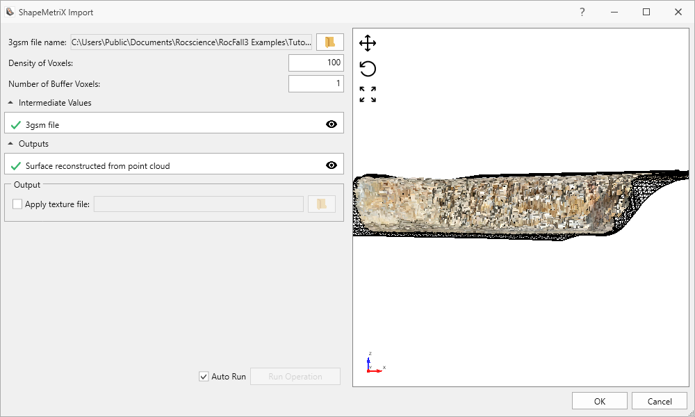
Slope Bench Face geometry preview in ShapeMetriX Import dialog Click OK, the following dialog will be displayed:
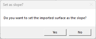
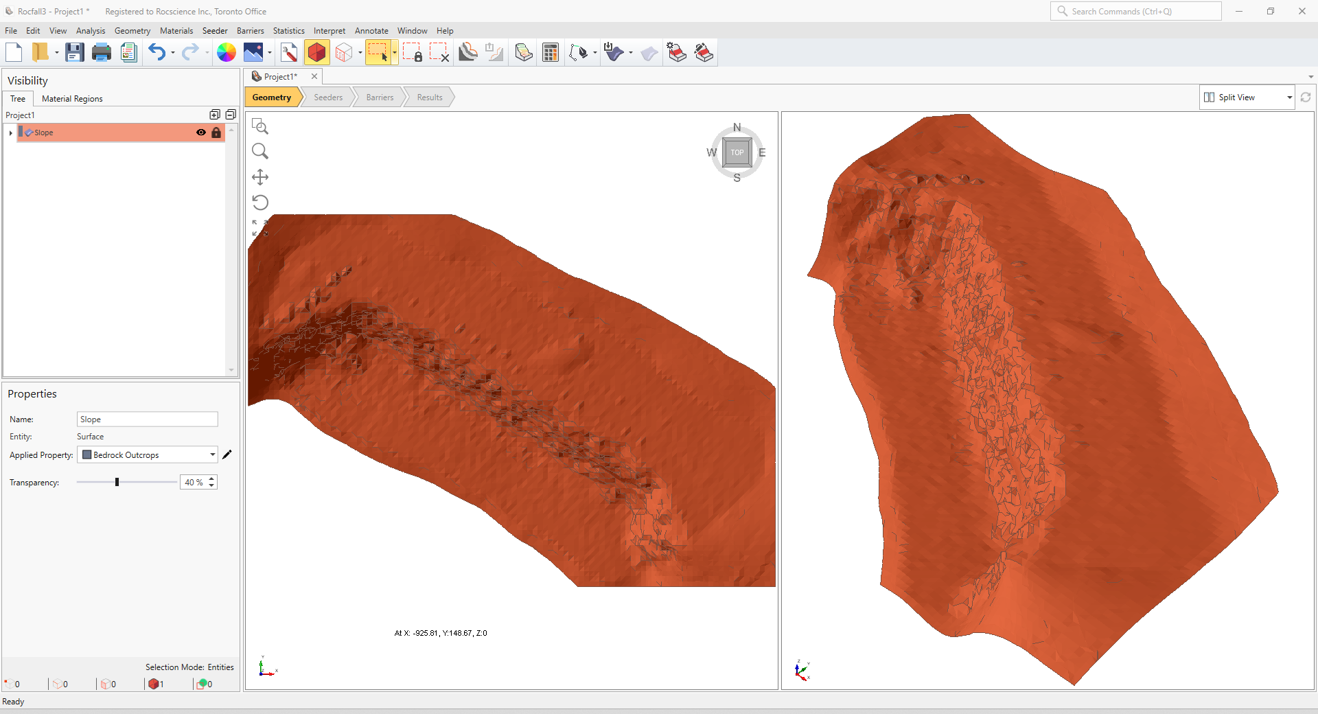
Set as slope surface dialog - Click Yes to set the imported ShapeMetriX slope geometry as the Slope.
- The geometry is imported into RocFall3 and added to the Visibility Tree. Click the Imported ShapeMetriX Geometry entity in the Visibility Tree. Notice in the Properties pane (below the Visibility pane) that the entity is imported as a Surface and that the Applied Property is Bedrock Outcrops.
3.4 Seeder Properties
For this tutorial, 200 rocks are seeded and assumed to fall due to blasting, which means they may have a non-zero initial velocity.
- Select Seeder > Define Seeder Properties

- For Seeder Property 1, navigate to the Number of Rocks tab and set the value to 200.
- Navigate to the Initial Velocity tab. See the table below for the Mean, Std. Dev., Rel. Min, and Rel. Max for the translational velocity, trend, and plunge. A Normal distribution is used for all parameters.
| Property | Distribution | Mean | Std. Dev. | Rel. Min. | Rel. Max. |
| Translational Velocity | Normal | 0.5 | 0.5 | 0.5 | 0.5 |
| Trend | Normal | 105 | 15 | 45 | 45 |
| Plunge | Normal | 0 | 30 | 90 | 90 |
3.5 Add Seeders
Add a point seeder to the model.
- Select Seeder > Add Point Seeder

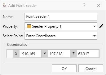
- In the Add Point Seeder dialog set:
- Name = Point Seeder 1
- Property = Seeder Property 1
- Select Point = Enter Coordinates. Enter the following coordinates (-910.169, 197.218, 63.317)
- Click OK.
A Point Seeder entity should appear in the Visibility Tree and on the slope.
Alternatively, a point seeder can be placed on the slope by left-clicking in the viewport.
4.0 Compute
When ready to compute:
- Select Analysis > Compute
 in the menu.
5.0 Results
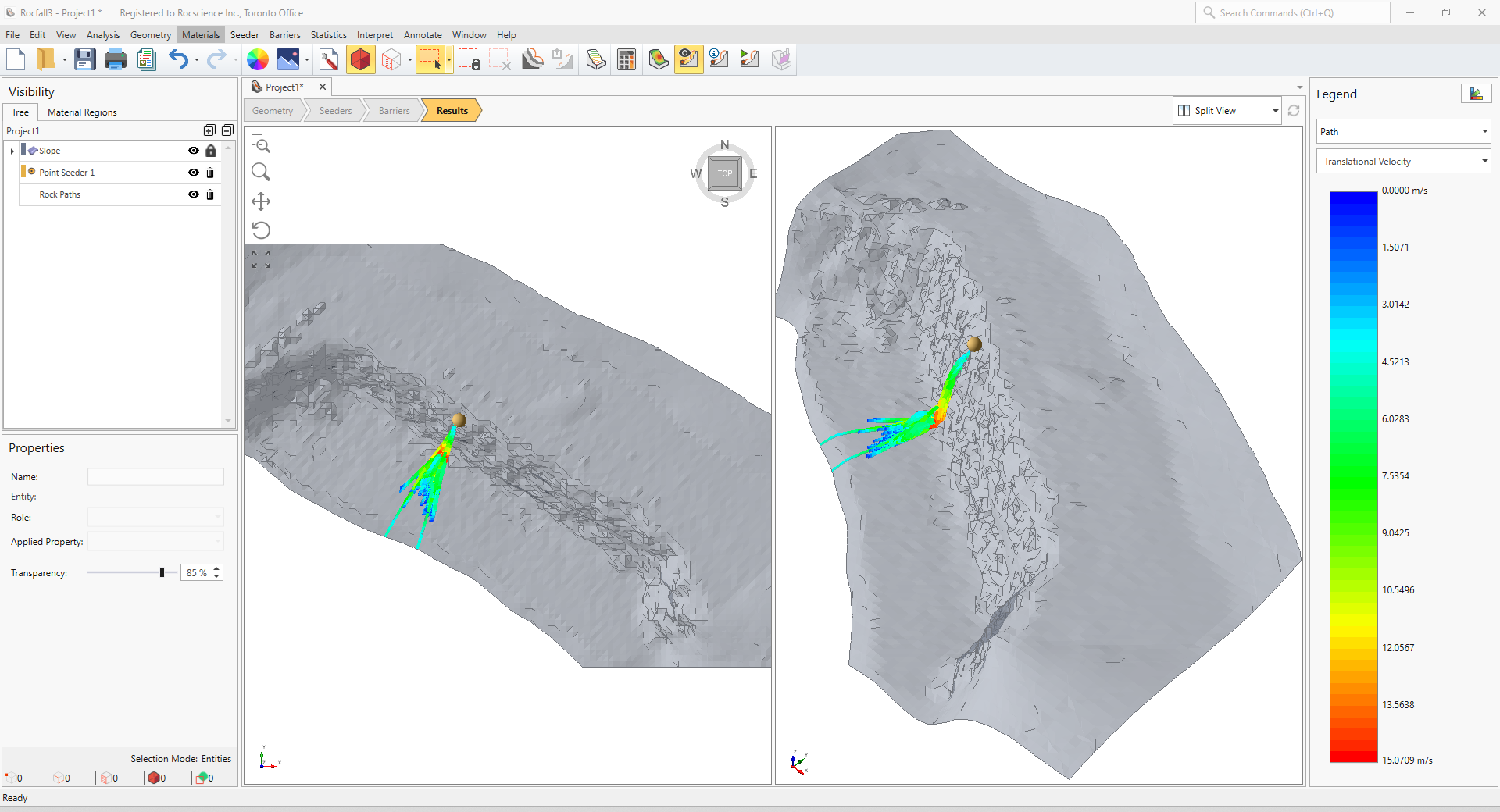
After the model has finished computing, navigate to the Results workflow tab to view results. By default, the results displayed are the translational velocity of each rock path, as shown in the legend on the right. Different results may be displayed using the legend options.
5.1 Runout Distance Graph
- Select Interpret > Graph Endpoints

Click OK in the Graph Endpoints dialog to plot the horizontal (XY) runout distance from the seeder location for all rock paths.
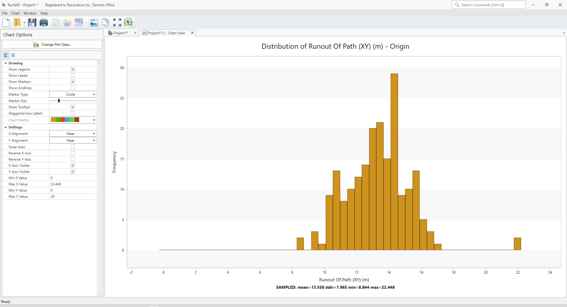
Histogram of horizontal (xy) runout distance from Point Seeder 1 for all rock paths The distribution of runout distances is now shown in a chart view. This histogram can be used to help determine barrier placements and evaluate any reference lines.
- Close the graph by clicking X on the view tab.
This concludes Tutorial 7.