3 - Import RocFall2 Model Tutorial

This tutorial provides an introduction on how to import a RocFall2 file, how to add Barriers to a RocFall3 model, and various analysis tools.

Topics Covered in this Tutorial:

• Import RocFall2 files
• Extrude 2D models
• Add Barriers
• Graph Barrier Results

Finished Product:

The finished product of this tutorial can be found in the Tutorial 03 RF2 import and barrier data file. All tutorial files installed with RocFall3 can be accessed by selecting File > Recent Folders > Tutorials Folder from the RocFall3 main menu.

1.0 Import a RocFall2 File

Let's import the RocFall2 Quick Start tutorial file:

1. Select File > Import > Import RocFall2 File.
2. Go to the Tutorials folder included with the RocFall3 install. The default location of this folder is C:\Users\Public\Documents\Rocscience\RocFall3 Examples\Tutorials. Select the Tutorial 03 RF2 file and click Open. The Import Rocfall2 Options dialog should open as follows:
   
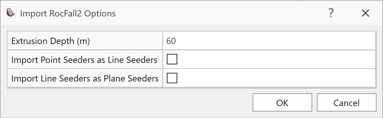
3. Enter 50 m for the Extrusion Depth, check the Import Point Seeders as Line Seeders option and enter 40 m for the Seeder Extrusion Depth.
4. Click OK.

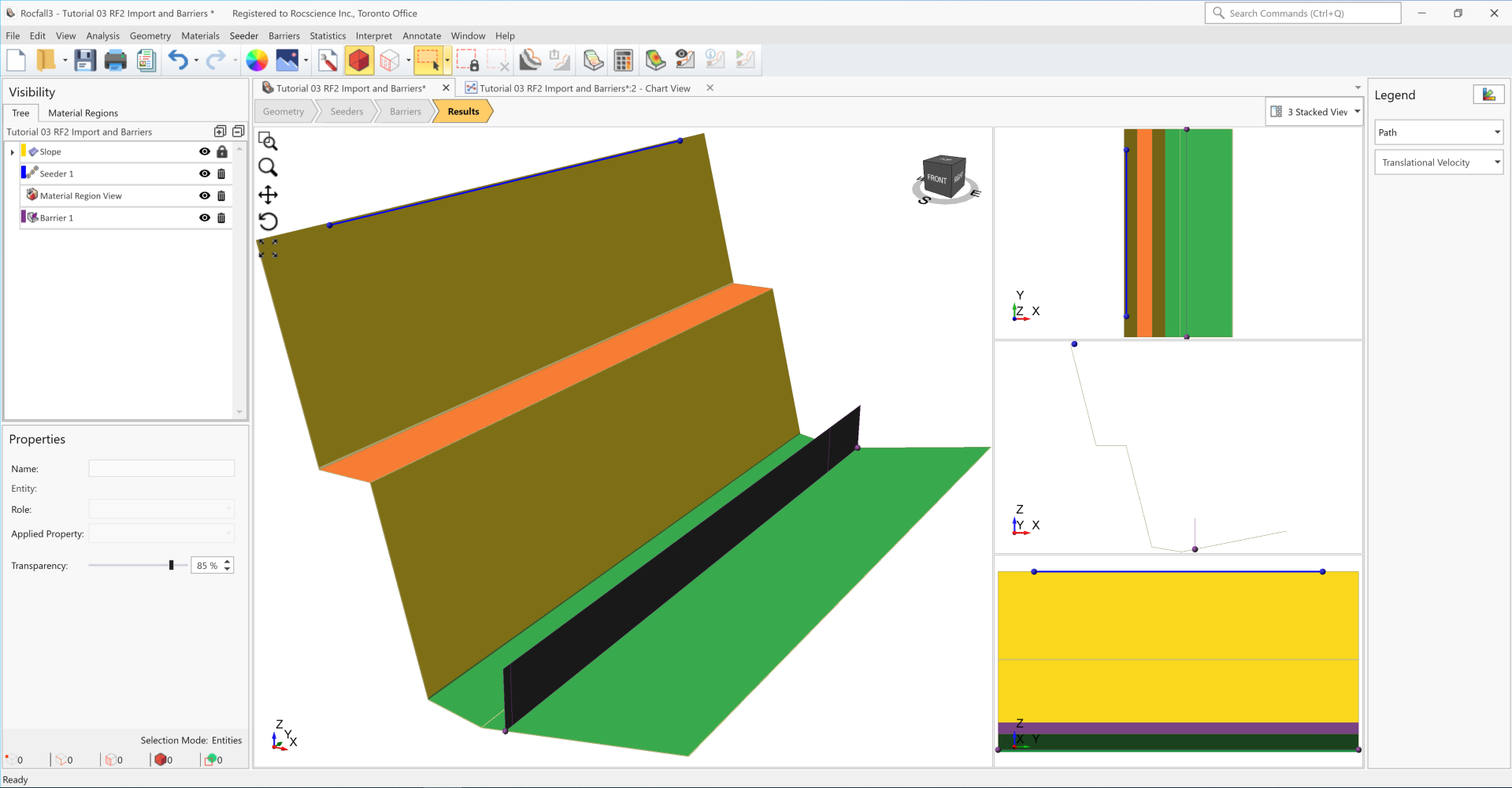
The imported model should include the extruded 2D geometry and all properties for the slope materials and seeders.

5. Select the Line Seeder entity from the visibility tree and click Edit from the Properties pane.
6. In the Edit Line Seeder dialog, change the geometry coordinates to (1,5,0) and (1,45,0) and click OK.

Open up the corresponding dialogs and observe the following:

• Analysis > Project Settings > Methods: Rigid Body Analysis Method
• Materials > Define Materials: Three slope materials (Type One, Type Two and Type Three) with statistical distributions:
  
  

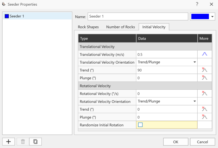
  Name	Normal Restitution	St. dev. / Rel.Min / Rel.Max	Dynamic Friction	St. dev. / Rel.Min / Rel.Max
  Type One	0.3 (Normal)	0.03 / 0.09 / 0.09	0.55 (None)	-
  Type Two	0.2 (Normal)	0.03 / 0.09 / 0.09	0.55 (None)	-
  Type Three	0.1 (Normal)	0.03 / 0.09 / 0.09	0.55 (None)	-

• Seeder > Define Seeder Properties: Seeder 1 property with statistical distribution for the initial translational velocity
  • In the Initial Velocity tab, uncheck Randomize Initial Rotation
    
    
    
  • Number of Rocks = 50
  • In the Rock Shapes tab, Group 1 with a mass of 1000kg and shapes using Extruded Polygon Square, Extruded Polygon Hexagon
  • In the Rock Shapes tab, Group 2 with a mass of 10000kg and shapes using Extruded Polygon Triangle, Extruded Polygon Octagon

1.1 Initial Compute

Save the model and run compute.

1. Select Analysis > Compute
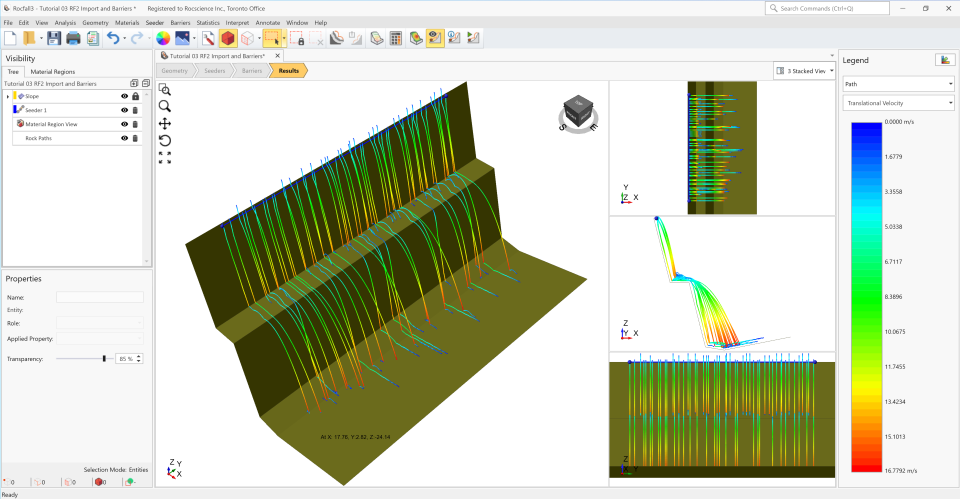
2. Click on the Results workflow tab

3. To view the rock paths, use the 3 Stacked Views option to visualize the rock paths from different perspectives. Select the Split View drop down menu located at the top right of the viewport, and select 3 Stacked View .
   
4. Select Interpret > Graph Endpoints and use the default options in the Chart Options dialog, and click OK.
   
   
   
   
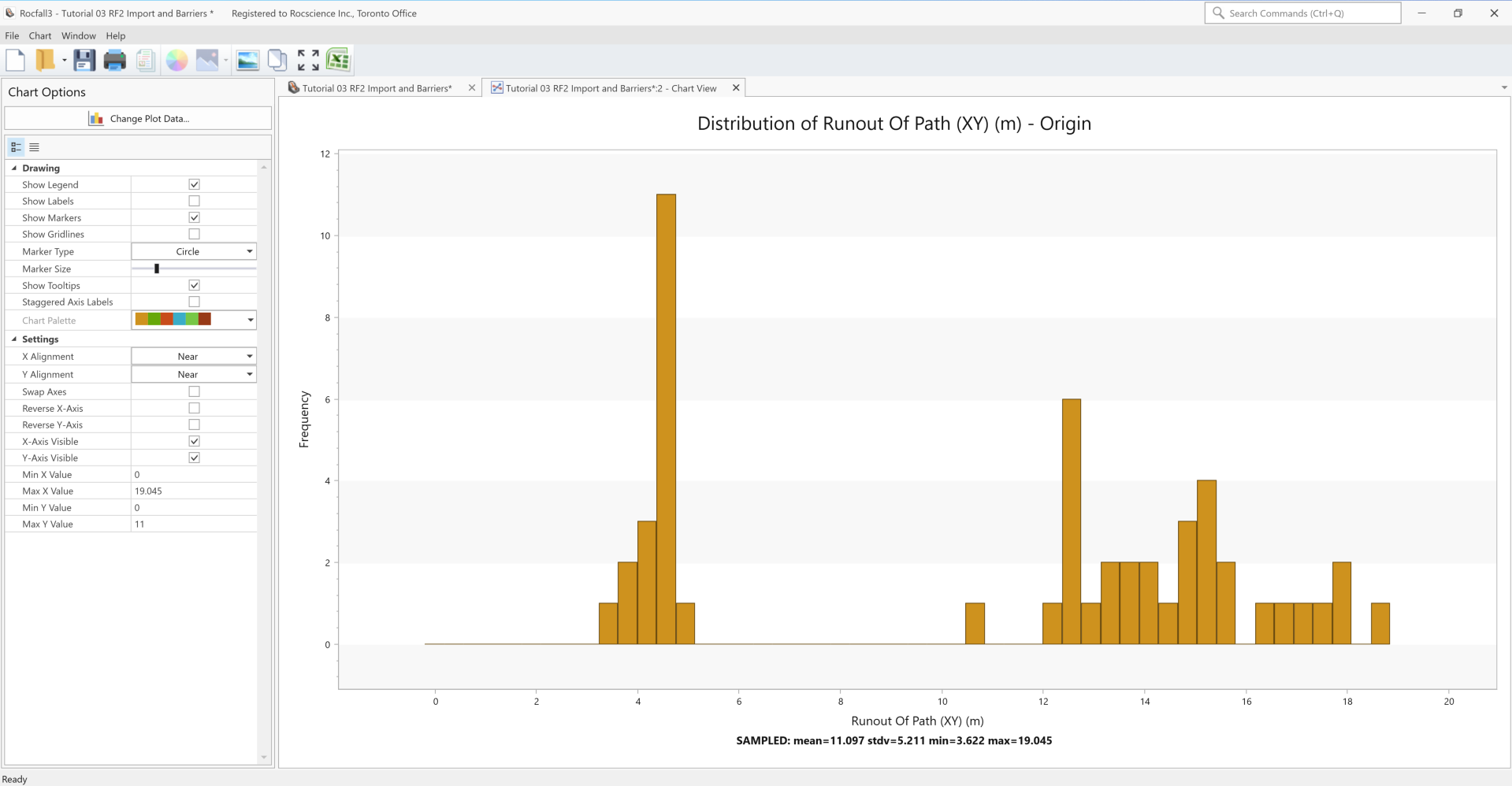
5. The next part of the tutorial is to add a barrier and to interpret barrier results. Before doing so, close the Endpoints graph using the close option X located on the right corner of the window tab, then Interpret > Clear Results to remove computed results.

2.0 Add Barrier

Barriers can be placed anywhere on the slope in RocFall3, and any number of barriers can be added to the model. A barrier in RocFall3 is defined with a height, an inclination, and a capacity. The barrier alignment is defined using a polyline, which means there can be flexibility in the geometry. A barrier can have a user-specified custom capacity (Custom Type barriers) or be chosen from the built-in barrier manufacturer library (Predefined Type barriers).

If a Custom Type is selected, the following inputs are required:

• Model Type: Custom or Infinite
• Capacity (for non-infinite type)

If a Predefined barrier is selected, the following inputs are required:

• Manufacturer barrier model
• Energy Level: MEL or SEL (when available)

To add a barrier, change to the Barriers workflow tab, then:

1. Select Barriers > Add Barrier
2. In the Add Barrier dialog, enter a height of 4 m. Keep the Default Barrier Property in the dropdown. The Default Barrier property can be viewed in detail by clicking on the pencil icon.
   
   
   
   
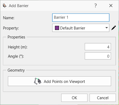
3. Click on Add Points on Viewport.
4. In the top right view, click on points close to (15,0) and (15,50). Don't worry about getting the exact points. Right-click and select Done when finished drawing the barrier. The points added can now be edited to the exact coordinates mentioned above.
5. Click OK in the Add Barrier dialog.

Barriers can also be added by converting from polylines. As an exercise, create a polyline with 2 vertices: (15,0,-24.68253968) and (15,50,-24.68253968). Select the polyline entity in the Visibility Tree. From the Barriers menu, select Add Barrier from Polyline. Follow the same steps from above to input the Height and click OK.

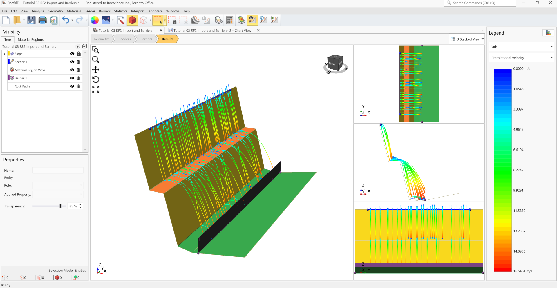
2.1 Compute

1. Select: Analysis > Compute
2. Click on the Results workflow tab and observe the path results. Most of the paths that went down the bench were caught by the barrier.
   

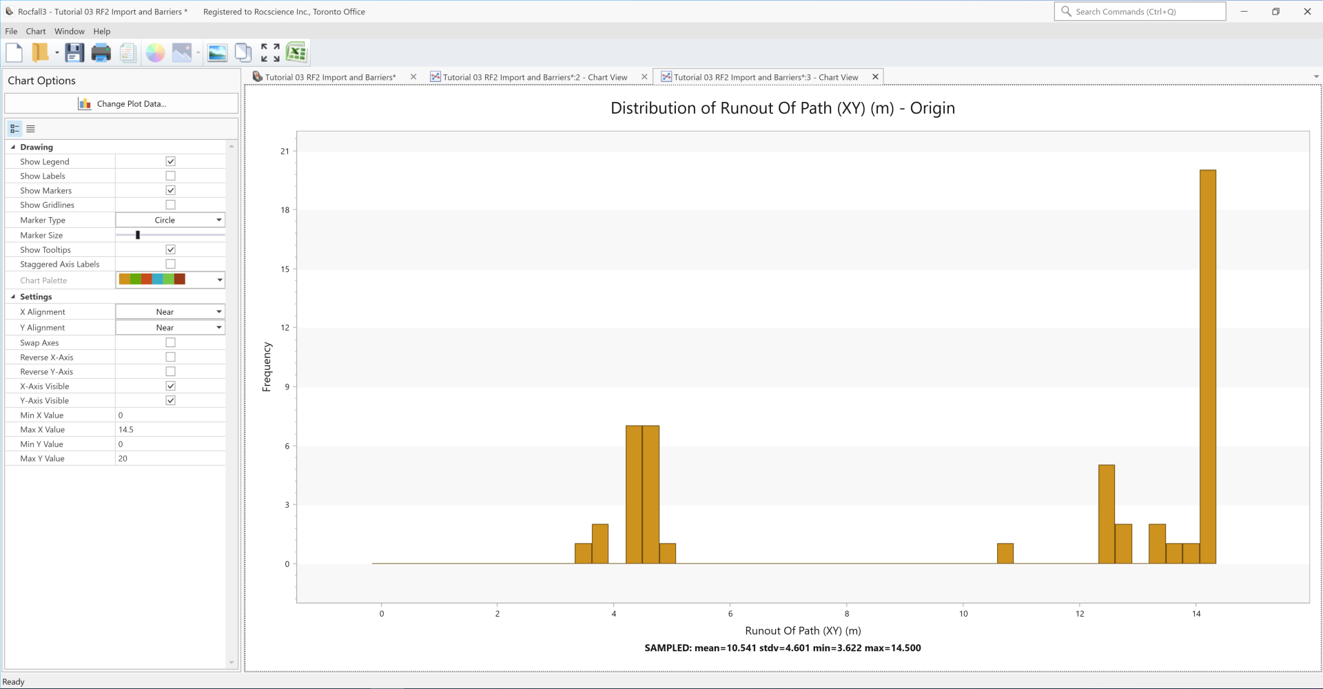
3. Select Interpret > Graph Endpoints and use the default options in the Chart Options dialog and press OK. The following histogram shows the distribution of horizontal (xy) runout distances from the seeder.
   
   
   

3.0 Graph Barrier Results

The following data types can be graphed for each barrier in the model. Note that results are only generated for rocks that came into contact with the selected barrier.

• Total Kinetic Energy
• Translational Kinetic Energy
• Rotational Kinetic Energy
• Translational Velocity
• Rotational Velocity
• Impact Height

To graph barrier data, select Interpret > Graph Barriers on the menu:

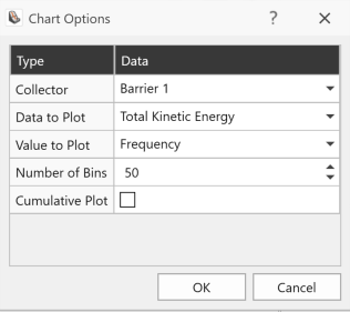
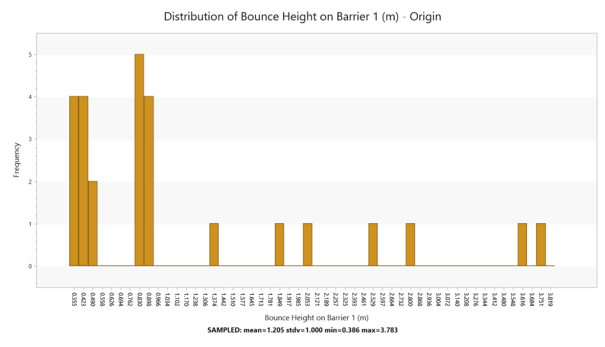
1. In the dialog, select Bounce Height for Data to Plot.
   
2. Leave Cumulative Plot unchecked for plotting a histogram.
3. Click OK.

Now let's graph the total kinetic energy of the rocks impacting the barrier:

1. In the same dialog, select Total Kinetic Energy for Data to Plot.
2. Check Cumulative Plot.
3. Click OK.

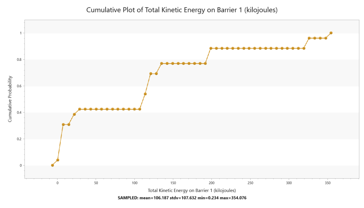
A sampler showing the percentile value becomes available when the mouse is hovered over the chart. Right-click on the plot to access exporting to Excel, copying the chart image or copying the data to clipboard for further post-processing.