1 - Getting Started Tutorial
This tutorial introduces the basic modelling and data interpretation features of RocFall3. RocFall3 is a 3D statistical rockfall analysis program designed to assist with the assessment of slopes at risk of rockfalls.
Topics covered in this tutorial:
- Importing a geometry file
- Defining material and seeder properties
- Applying/editing seeders
- Creating material regions
- Computing
- Interpreting
Finished product:
The finished product of this tutorial can be found in the Tutorial 01 Getting Started.r3DModel data file. All tutorial files installed with RocFall3 can be accessed by selecting File > Recent Folders > Tutorials Folder from the RocFall3 main menu.
Want to watch the video version of the tutorial? Check it out here:
1.0 Model
Start RocFall3 by selecting Programs > Rocscience > RocFall3 > RocFall3 from the Windows Start menu. RocFall3 automatically opens a new blank document, which allows you to begin creating a model immediately. If the RocFall3 application window is not already maximized, maximize it now so the full-screen space is available for use.
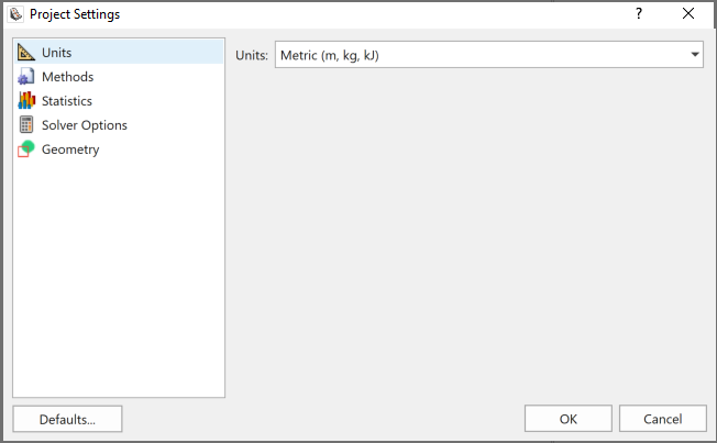
1.1 Project Settings
The Project Settings dialog is used to configure the main analysis parameters of the model. To open the dialog, select Project Settings on the toolbar or the Analysis menu. For the tutorial, we'll use default parameters.
- Select: Analysis > Project Settings

1.1.1 Analysis Type
- Select the Methods tab. In RocFall3, there are two Analysis Types to choose from: Lump Mass and Rigid Body.
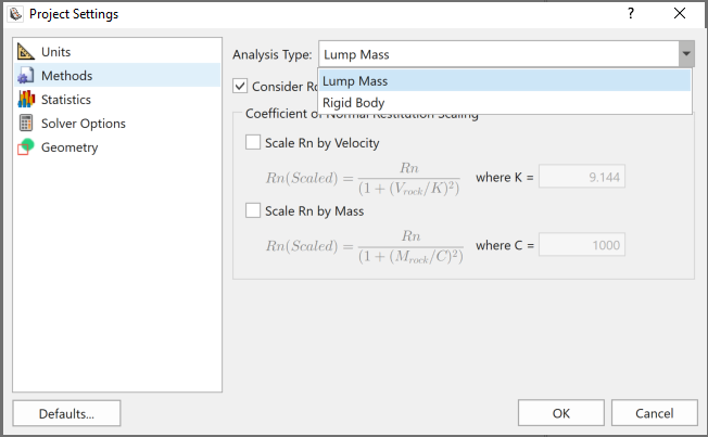
The default analysis method is Lump Mass. With the Lump Mass method, all rocks are assumed to be infinitely small point masses. We will be using the Lump Mass method for this tutorial.
The Rigid Body analysis method explicitly considers the rock shape. The Rigid Body method is covered in later tutorials.
1.1.2 Engine Conditions
- Select the Solver Options tab.
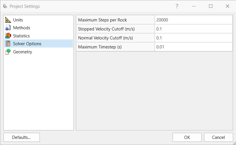
Solver options (engine stopping conditions) Solver options are engine-stopping conditions. A rock stops moving when it meets one of these conditions. For more help on engine stopping conditions, see Engine Stopping Conditions Settings in RocFall3. - For this tutorial, use default settings.
- Click OK.
1.2 Import Geometry
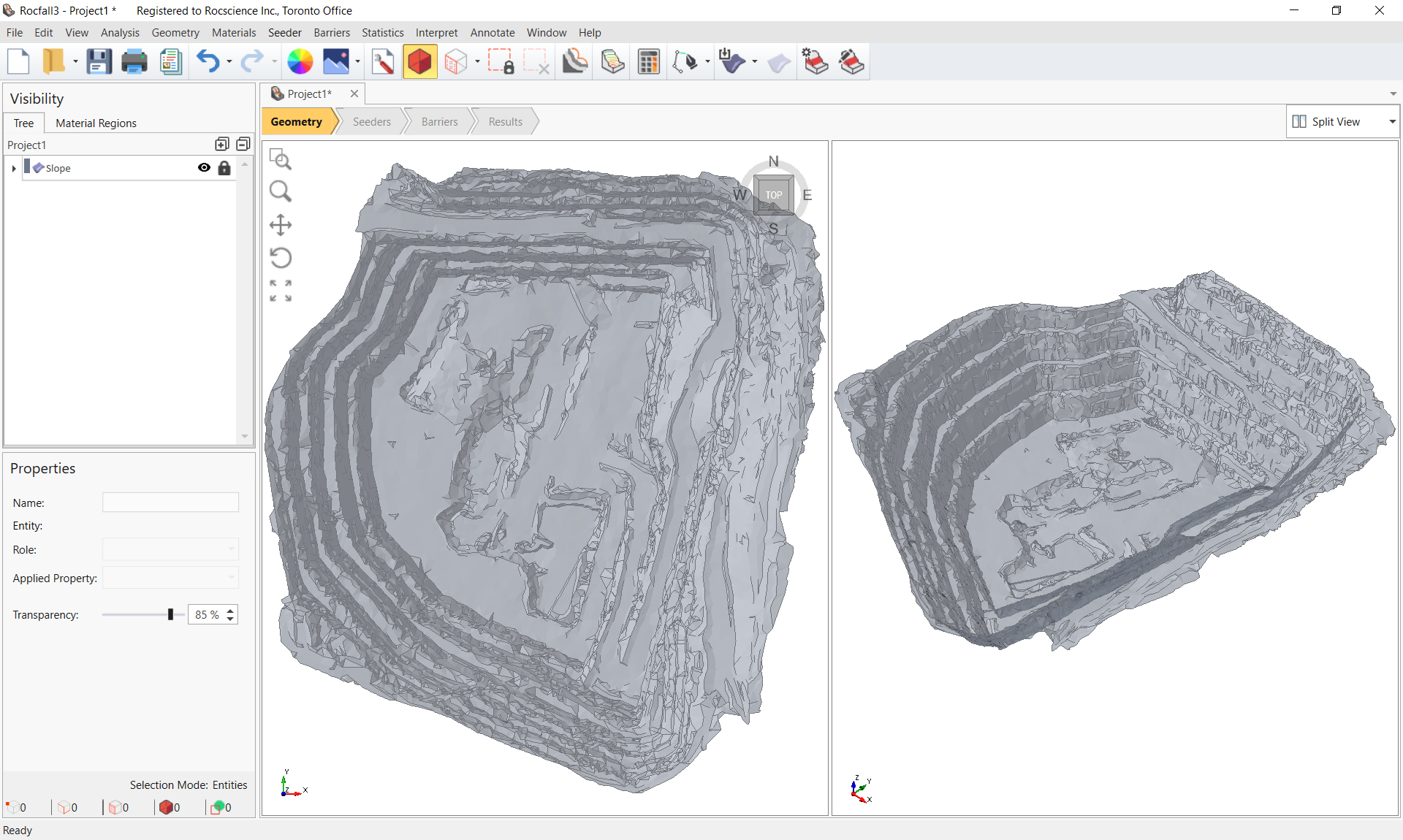
In RocFall3, the slope geometry can be created from points, lines, or surfaces, as long as the file being imported is of a common geometry file type. In addition, a RocFall3 model can be extruded from an existing RocFall2 file, imported from an RS3/Slide3 File, or imported from satellite data (digital elevation model from Import Terrain). In this tutorial, a provided .obj file is imported.
- Select File > Import > Import Geometry
 or Geometry > Import/Export > Import Geometry .
 - Open the provided Tutorial 01.obj file in the Tutorials Folder. By default, the installation program puts the files in: C:\Users\Public\Documents\Rocscience\RocFall3 Examples\Tutorials
- The Import Geometry dialog displays a preview of the geometry. Select the Mesh object and click on Post-Processing.
- The Post-Processing step provides the option to simplify and repair the geometry. The supplied sample geometry file has already been modified and fixed for this tutorial. Typically, both simplify and repair are recommended when importing raw geometry for optimal computing performance.
- Click Done.
- A prompt appears to set the imported surface as the slope. Click Yes.
1.3 Material Properties
- Select Materials > Define Materials
 . This opens up the Define Material Properties dialog. The program has 3 built-in materials.
- Rename the first material to Hard and change the mean Normal Restitution to 0.5 and Tangential Restitution to 0.9.
- Click on the Stats
 button for Tangential Restitution and change the Rel. Max to 0.1 so that the absolute range is 0.78 to 1.0.
The Hard material property values should look like the following when the All Statistics button is clicked:
| Property | Distribution | Mean | Std. Dev. | Rel. Min. | Rel. Max |
| Normal Restitution | Normal | 0.5 | 0.04 | 0.12 | 0.12 |
| Tangential Restitution | Normal | 0.9 | 0.04 | 0.12 | 0.1 |
| Friction Angle (°) | None  | 30 | - | - | - |
- Select the second material property in the list and rename it to Soft.
- Change the mean Normal Restitution to 0.3.
- Make sure the mean Tangential Restitution is 0.8 and that the standard deviation for the two restitutions are both 0.04 and the relative min and max are all 0.12.
- Keep the Friction Angle at 30 degrees with no distribution.
- Click OK.
1.4 Define Material Regions
- Select Materials > Add New Material Region
 . Notice that you're now on the Material Regions tab in the left Visibility pane.
- Select the Soft material property and click OK.
- Now in the Draw Polyline mode, roughly trace (left-click) around the bottom of the pit to assign this polygonal region with the Soft material property. Alternatively, to use the exact coordinates of the material region as adopted in this tutorial model, open the provided Tutorial 01 Material Region.txt file in the Tutorial Folder. Select the Edit Table button located on the Draw Polyline pane, open the Edit Polyline dialog, import the points.
- When done drawing the material region or importing the coordinates, right-click and select Done.
The screen should look like the following:
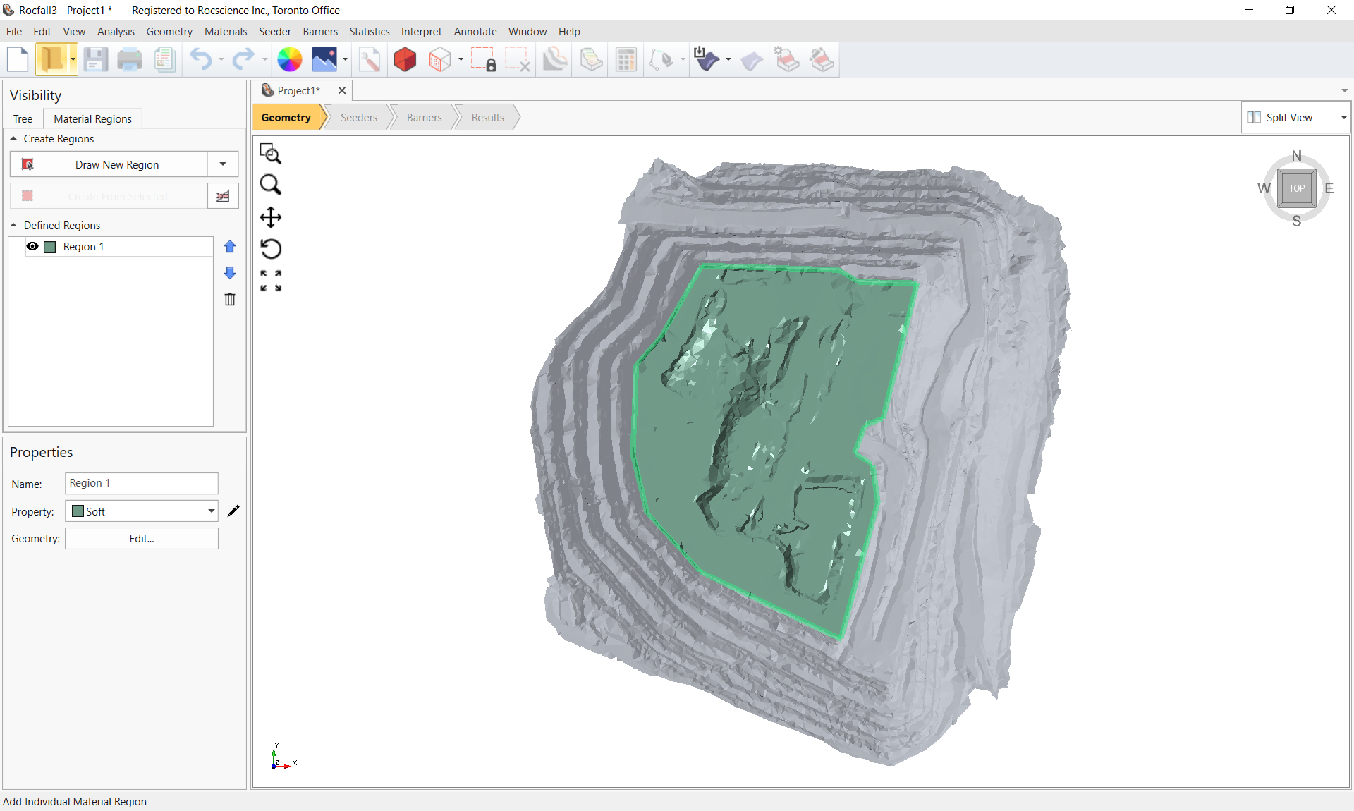
The coordinates that define the polygon material region can be viewed by clicking on the Edit... button in the Properties pane.
Take note that the rest of the slope has the shading of the first (Hard) material. By default, if no material region is explicitly assigned, the first material property on the list is assigned to the entire slope.
- Click on the Tree tab in the left pane to exit the Material Regions mode and to return to the Visibility Tree.
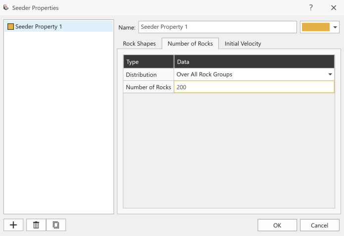
1.5 Seeder Properties
- Select the Seeders workflow tab
- Select Seeder > Define Seeder Properties
 to open the Seeder Properties dialog.
 - For Seeder Property 1, change the Number of Rocks to 200. Keep all other default values, so all rocks would be free falling from the seeder location.
- Click on the Add
 button to add a new seeder property.
 - In Seeder Property 2, change the Number of Rocks to 20.
- In the Initial Velocity tab, enter 1.5 m/s for the Translational Velocity.
- Click on the Stats button, change the Distribution to Normal and enter a Std. Dev. of 0.3.
- Click on the 3x button to auto set Rel. Min and Rel. Max to 0.9 (3x std. dev.).
- Click OK.
- In the Translational Velocity Orientation dropdown, select Trend/Plunge. Enter a Trend angle of 225 deg, defined clockwise from the y-axis.
- Click on the Stats button, change the Distribution to Normal and enter a Std. Dev. of 5.
- Click on the 3x button to auto set Rel. Min and Rel. Max to 15 (3x std. dev.)
- Click OK to save and exit the Seeder Properties dialog.
1.6 Add Seeders
Add a line and a point seeder to this model.
- Select Seeder > Add Line Seeder

- In the Add Line Seeder dialog, select Seeder Property 1 that has 200 rocks for the Property.
- For the Elevation (Z Value) dropdown, select Height Above Surface and enter 5 m.
- Click on Add Points on Viewport. In the viewport displaying the top view, trace (left-click) long the crest of the 2nd uppermost bench (see yellow polyline in below image).
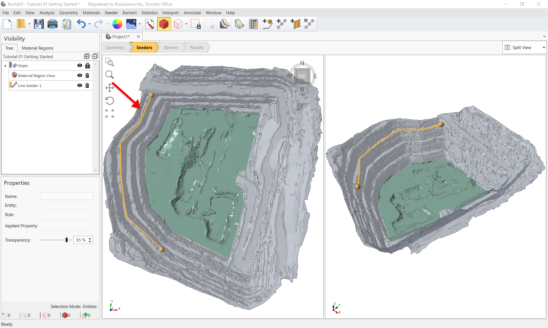
Line seeder on second uppermost bench crest - When done drawing the line seeder, right-click and select Done, to return to the Add Line Seeder dialog. The Add Line Seeder dialog should look like the following:
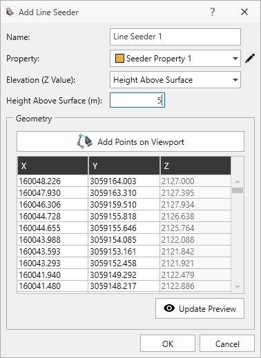
Add Line Seeder dialog - Click OK to save and exit the Add Line Seeder dialog.
For exact line seeder coordinates, open the provided Tutorial 01 Line Seeder.txt file in the Tutorial Folder, and import the points with the following steps:
- Create a polyline using Geometry > Draw Polyline

- In the Draw Polyline pane, select the Edit Table button, and then select the Import button located on the bottom-left corner of the dialog.
- Import the provided file.
- Close the dialog by clicking Ok, and then right-click and select Done.
- Convert the polyline to a line seeder by selecting the polyline entity in the Visibility Tree, and then Seeder > Add Line Seeder from Polyline in the menu.
- Set Height Above Surface to 5m, and then click OK to close the Add Line Seeder dialog.
Next, to add the point seeder:
- Select Seeder > Add Point Seeder

- Select Seeder Property 2 in the Property dropdown.
- Select Enter Coordinates in the Select Point dropdown.
- Enter the coordinates 160366, 3059160, 2099 in the Coordinates area.
- Press OK.
2.0 Compute
- When ready to compute, select Analysis > Compute
 in the menu.
3.0 Results and Interpretation
3.1 Rock Path Contours
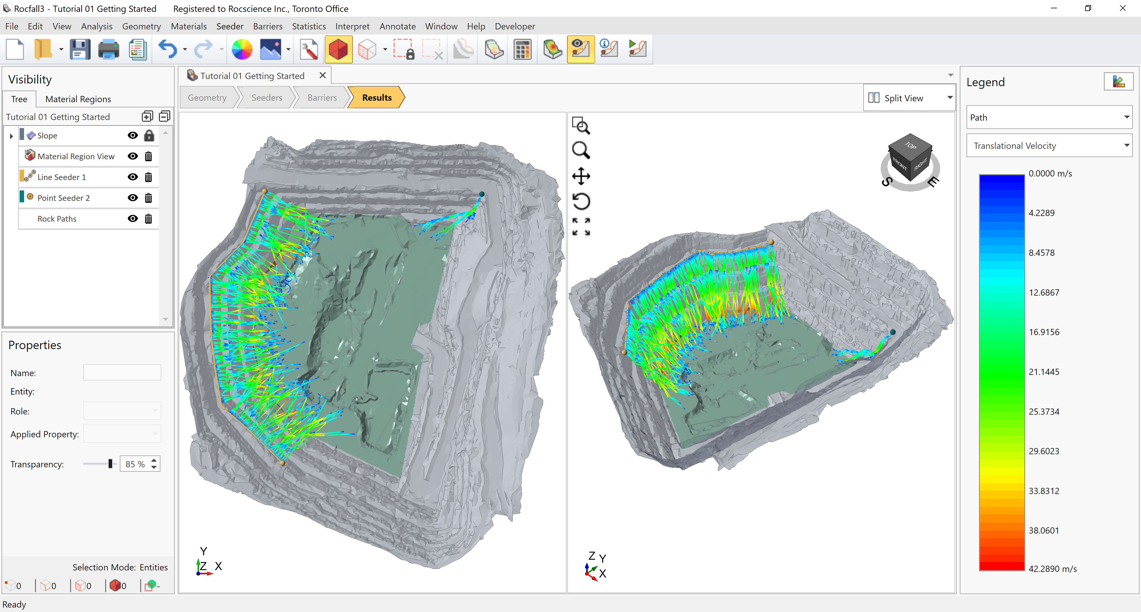
- Select the Results workflow tab to see the computed results.
By default, rock paths are shown with contours for the translational velocity. This is because in the Legend pane on the right, results are shown for the "Path" and the "Translational Velocity" data type.
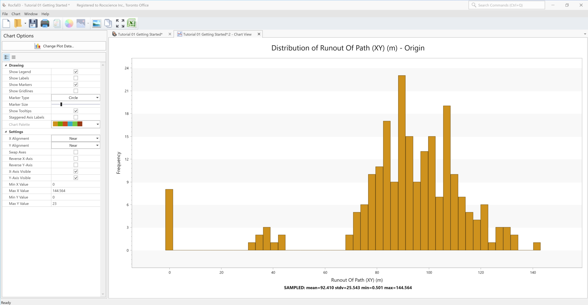
3.2 Runout Distance Graph
- Select Interpret > Graph Endpoints

- Click OK in the Graph Endpoints dialog to plot the horizontal (XY) runout distance from the seeder location for all rock paths.
- Close the graph by clicking X on the view tab.
3.3 Runout Distances Calculated using a Reference Line
In RocFall3, runout distances can be calculated with respect to a reference polyline. There are 2 ways to assign a reference polyline: 1) by selecting a pre-existing polyline; or 2) by drawing a new polyline from the Graph Endpoints dialog. We will select a pre-existing polyline to calculate runout distances.
Selecting a pre-existing polyline as the reference line:
- Select Geometry > Draw Polyline
- Draw the polyline in the viewport or insert coordinates with the following steps.
- Select the Edit Table button in the Draw Polyline Pane, and then select the Import button located at the bottom-left corner of the Edit Polyline dialog.
- Open the provided Tutorial 01 Reference Line.txt file in the Tutorials folder. Alternatively, you can save the .txt file by right-clicking the link and selecting Save Link As.
- Close dialogs by pressing OK twice, and then right-click on the viewport and select Done to exit the polyline drawing mode.
- Name the polyline "Reference Line".
- Select Interpret > Graph Endpoints
- In the Graph Endpoints dialog, select the Reference line option, and then select the defined polyline, "Reference Line".
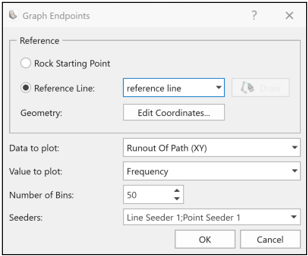
Graph Endpoints dialog with a reference line selected - Click OK, and a histogram of the rock runout distances calculated from the reference line should appear.
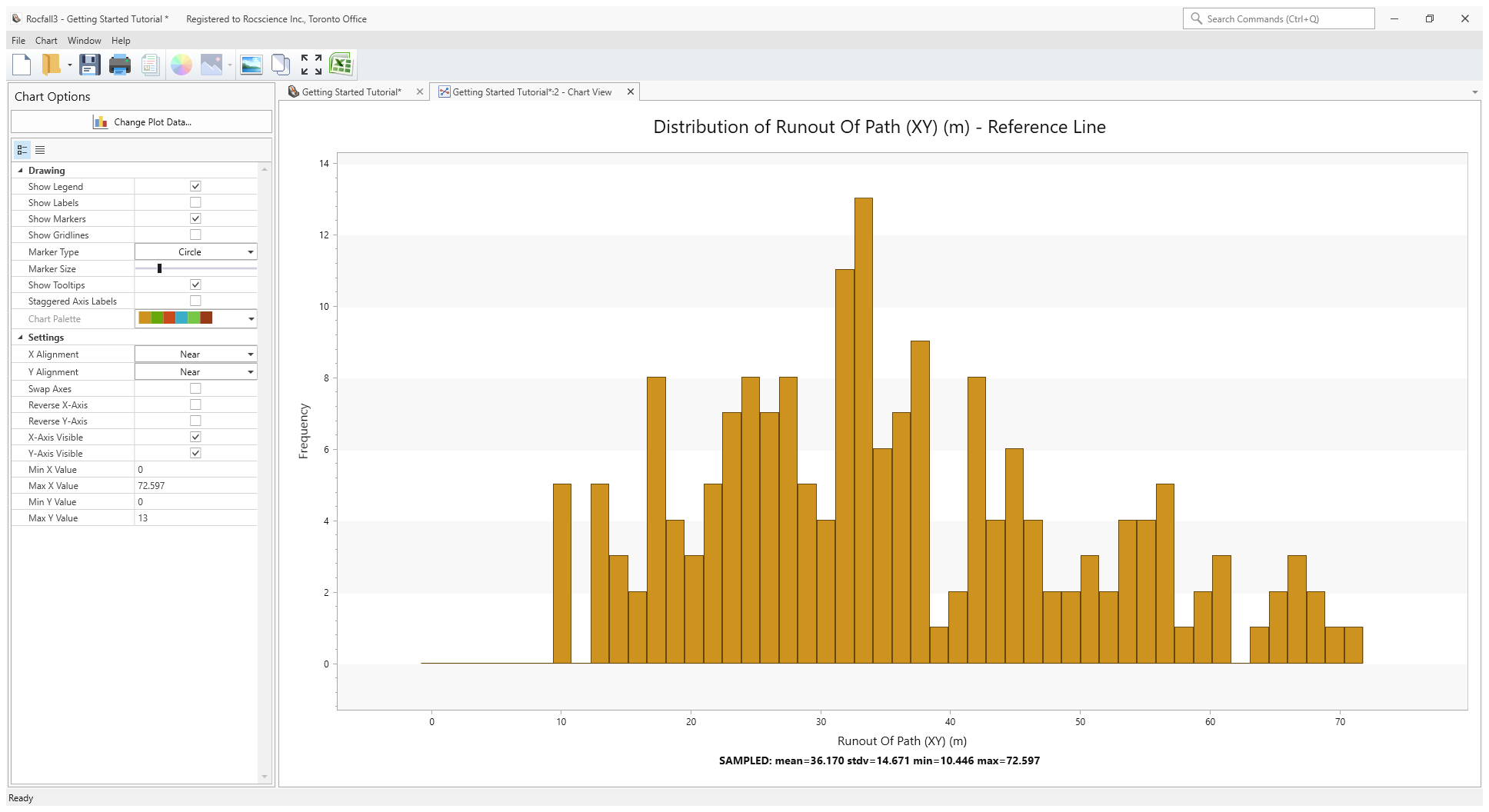
Histogram of horizontal (xy) runout distances calculated with respect to a reference line
3.4 Surface Heat Map
- Select Interpret > Create Surface Heat Map

- For best viewing results, turn off the Rock Path Results entity by left-clicking on the Toggle Rock Path Results
 toolbar option.
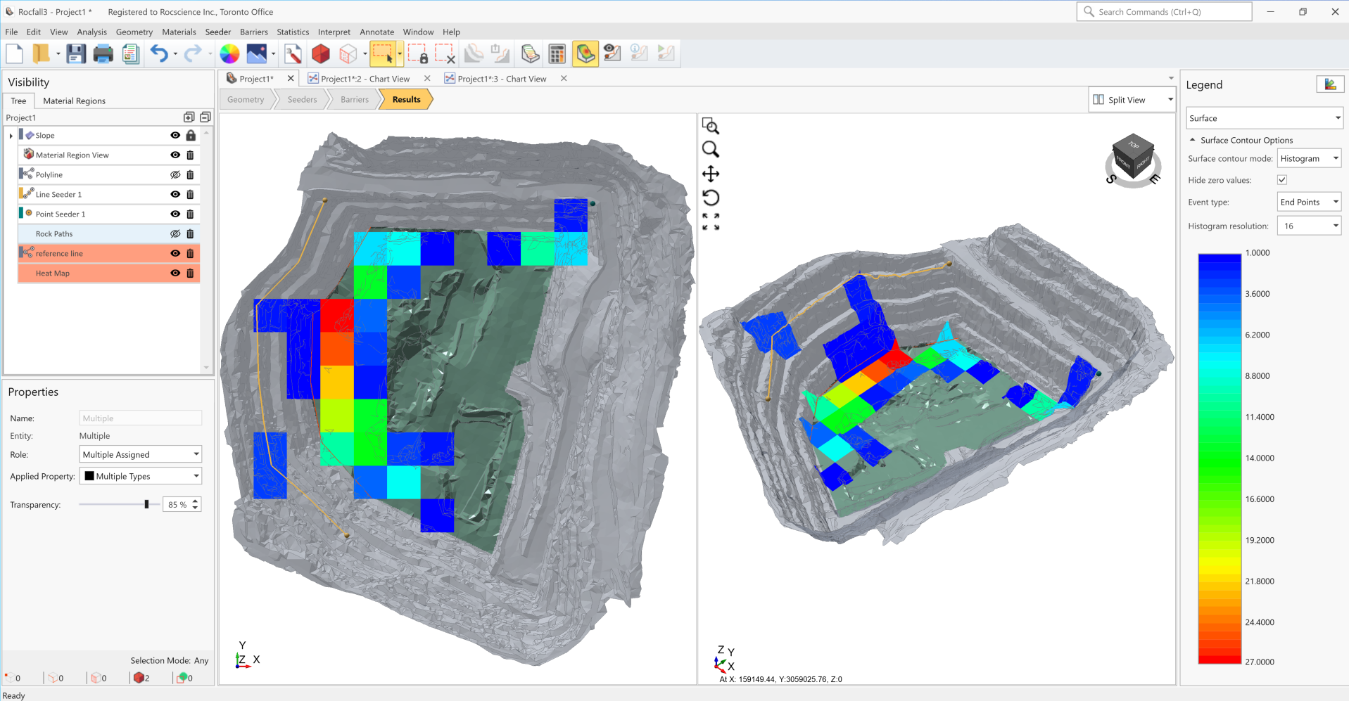
Several data types can be plotted on a surface heat map, including End Points, Impact Points, as well as Kinetic Energies and Bounce Heights.
For more information on the surface heat map, see this article: Create Surface Heat Map
3.5 Rock Path Information
- Select Interpret > Rock Path Information

If the option is disabled, you must have turned off the rock paths when looking at the Heat Map. Simply turn on the rock paths again by selecting the Toggle Rock Path results  option on the toolbar, and select the Rock Path Information
option.
option on the toolbar, and select the Rock Path Information
option.
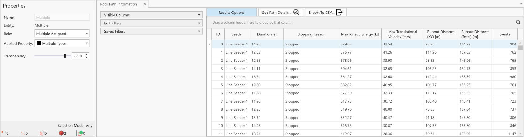
A tabulated summary of the rock paths is provided. The data can be sorted and/or filtered by any of the column headers. For example, click on the Max Kinetic Energy header cell and the table is sorted from smallest Max Kinetic Energy to largest. Click on the header cell again to reverse the sort from the largest Max Kinetic Energy to the smallest.
- Next, click on Edit Filters in the pane to the left of the rock information table and select Point Seeder 1 only.
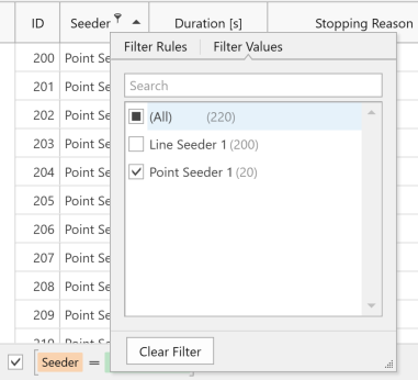
The table and the viewports now should only show rock paths from the point seeder. The filter can be cleared by unchecking the checkbox at the bottom of the table. The filter can be edited by clicking on the pencil icon. The filter can also be edited by expanding the Edit Filters option to the left of the table. In the Runout (XY) option at the bottom, drag the slider to see only the paths with horizontal runout distances that are within the specified range.
- To the left of the table, click to expand the Saved Filters option. Click on the Save Filter button at anytime to save the current filter setup for later use.
We'll leave it as an exercise for the user to explore all the table and filtering customization options.
3.6 Animate Rock Paths
A very useful feature of RocFall3 is the ability to animate the rocks as they fall and interact with the slope.
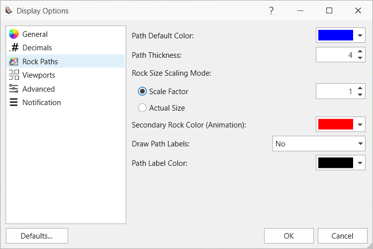
By default, rocks are animated with their actual size, calculated from inputs for the mass and density. The rock sizes could be very small compared to the slope size. A Scale Factor can be applied to increase the size of the animated rocks.
- Right-click anywhere in the viewport and select Display Options

- Select the Rocks Paths tab and set the Rock Size Scaling Mode to Scale Factor. Use a value as 1 and click OK.
Options to change the size of animated rocks - Select Interpret > Animate Rocks

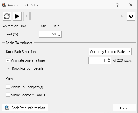
Rocks can be animated one at a time or all at the same time.
This concludes the tutorial. You are now ready for the next tutorial: Terrain Generator and Image Segmentation.