Finite Element Groundwater Seepage

1.0 Introduction

RS2 can be used to carry out finite element groundwater seepage analyses for saturated/unsaturated, as well as steady-state (or transient) flow conditions.

The model used in this tutorial used consists of a basic, steady-state groundwater seepage analysis integrated with stress analysis. This tutorial will focus on the results of the analysis; after a groundwater seepage analysis is computed, the results (pore pressures), are automatically used in the RS2 stress analysis to calculate effective stress.

The seepage analysis capability in RS2 can also be used as a standalone groundwater program, independently of the stress analysis functionality of RS2.

2.0 Constructing the Model

1. Select: File > Recent Folders > Tutorial Folder
2. Open: Finite Element Groundwater Seepage (Initial)

In this starting file, the project settings have been defined (Groundwater conditions = Steady State FEA), the external boundary has been created, units set to Metric (stress as MPa), and material and hydraulic properties defined.

2.1 Ponded Water Load

An important point to remember when defining an RS2 model which includes Ponded Water and both a groundwater seepage analysis and a stress analysis are used: the weight of the Ponded Water must be defined by adding a Ponded Water distributed load to the model.

The total head boundary conditions that you use to define the hydraulic boundary conditions DO NOT define the weight of the ponded water. Conversely, the Ponded Water distributed load DOES NOT define the total head boundary conditions required by the groundwater analysis.

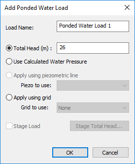
The Ponded Water load is defined as follows:

1. Select: Loading > Ponded Water Loads > Add Ponded Water Load
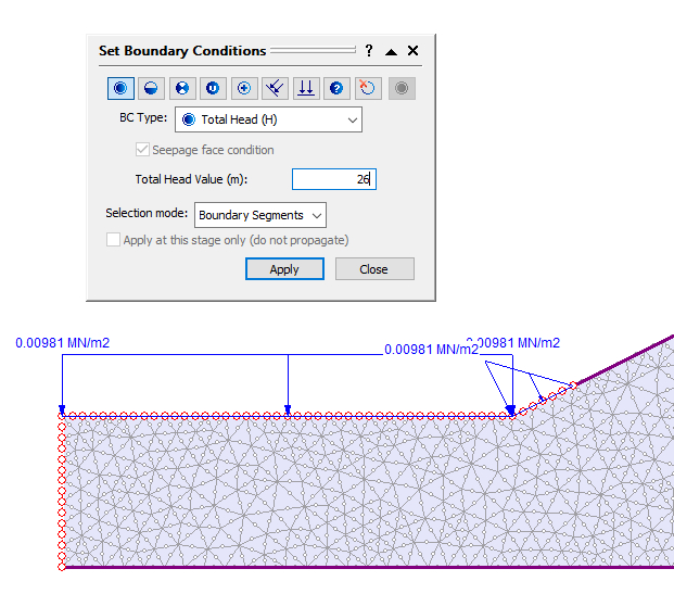
2. In the Add Ponded Water Load dialog, enter Total Head = 26m and press OK.
   
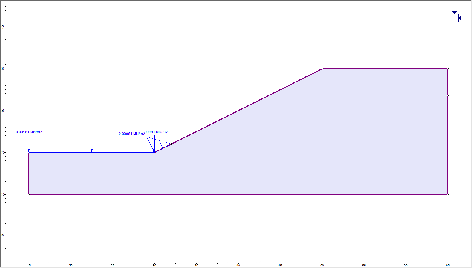
3. Select the slope segment between the vertices at (15,25) and (30,25) and the slope segment between vertices (30,25) and (32,26).
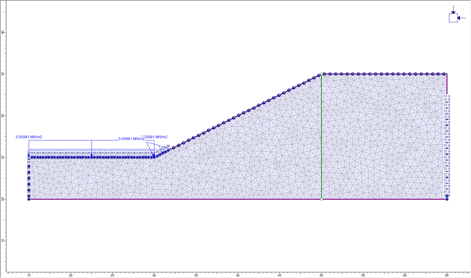
4. The ponded water load will be added to the model and is represented by blue arrows applied normal to the selected boundary segments.
RS2 automatically determines the magnitude of the load based on the value of Total Head, the elevation of the line segments, and the unit weight of water entered in the Project Settings dialog.

The model should appear as in the following figure:

2.2 Field Stress

A surface model usually requires Gravity Field Stress.

1. Select: Loading > Field Stress
2. Set the Field Stress Type to Gravity and turn on the option "Use actual ground surface".
3. Select OK.

2.3 Mesh

Now generate the finite element mesh:

1. Select: Mesh > Mesh Setup
2. Change the Mesh Type to Uniform. Leave the default element type (6 Noded Triangles) and enter number of elements = 2500.
3. Click the Discretize button followed by the Mesh button.
   
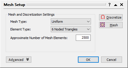
4. Close the Mesh Setup dialog by selecting the OK button.

2.4 Hydraulic Boundary Conditions

1. Select: Groundwater > Set Boundary Conditions

The Set Boundary Conditions dialog will appear. This dialog allows the definition of the hydraulic boundary conditions for groundwater analysis.

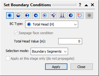
Let’s first set the Total Head boundary conditions:

2. Make sure the Total Head boundary condition option is selected in the Set Boundary Conditions dialog, as shown above.
3. In the dialog, enter a Total Head Value = 26 meters. Also make sure the Selection Mode is set to Boundary Segments.
4. Now select the desired boundary segments by clicking on them.
5. Click on the three segments of the external boundary indicated in the following figure. (i.e. the left edge of the external boundary, and the two segments at the toe of the slope). To better see the boundary conditions, use the visibility tree on the left side of the screen to hide the ponded water load.
   
6. When the segments are selected, right-click the mouse and select Done Selection. A boundary condition of Total Head = 26 meters is now assigned to these line segments.
The hatch pattern represents ponded water which is defined by the Total Head boundary condition of 26 meters on the selected segments.
7. Now enter a Total Head Value = 31.8 meters in the dialog. Select the lower right segment of the external boundary, as shown below. Right-click and select Done Selection.
   
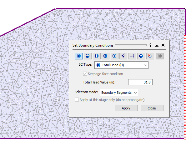
   The Total Head boundary conditions represent the elevation of the phreatic surface (ponded water) at the left of the model (26 m), and the elevation of the phreatic surface at the right edge of the model (31.8 m).
   Now we need to assign the Unknown (P=0 or Q=0) boundary condition to the upper two segments of the slope.
8. In the Set Boundary Conditions dialog, select the Unknown (P=0 or Q=0) boundary condition option.
   
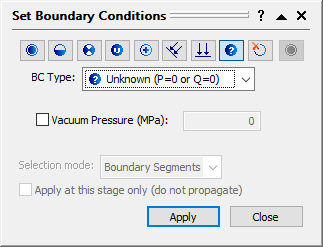
9. Select the upper two segments of the slope, as shown below. Right-click and select Done Selection.
   

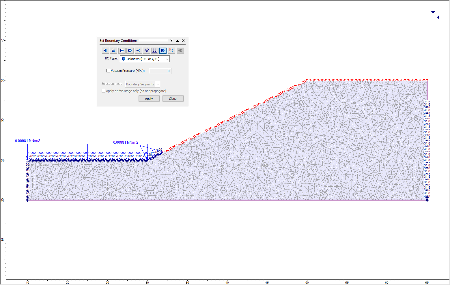
The necessary hydraulic boundary conditions are now assigned.

2.5 Discharge Section

A Discharge Section allows the user to compute the volumetric flow rate through a user-defined line segment. Let's add a Discharge Section to the model.

1. Select: Groundwater > Add Discharge
2. Right-click the mouse and make sure the Snap options are enabled
3. Click the mouse on the vertex at the crest of the slope at (50,35)
4. Click the mouse at the point (50,20) on the lower edge of the external boundary to create a vertical discharge section between the crest of the slope and the lower edge of the model, as shown in the figure below:
   

2.6 Stress Analysis Boundary Conditions

Although this tutorial is primarily concerned with how to define a groundwater seepage analysis model, the stress analysis aspects of the model will also be discussed, since in many cases, both analyses will be performed simultaneously.

First we have to free the segments of the external boundary representing the slope surface.

1. Select: Displacements > Free Displacements
2. Select the four line segments defining the ground surface of the slope.

The slope surface is now free, however, this process has also freed the vertices at the upper left and upper right corners of the model. Since these edges should be restrained, we have to make sure that these two corners are restrained.

We can use a right-click shortcut to assign boundary conditions:

3. Right-click the mouse directly on the vertex at (15,25).
4. From the popup menu select the Restrain X, Y option.
5. Right-click the mouse directly on the vertex at (65,35).
6. From the popup menu select the Restrain X, Y option. The restraint boundary conditions are now correctly applied.

The completed model should look like this: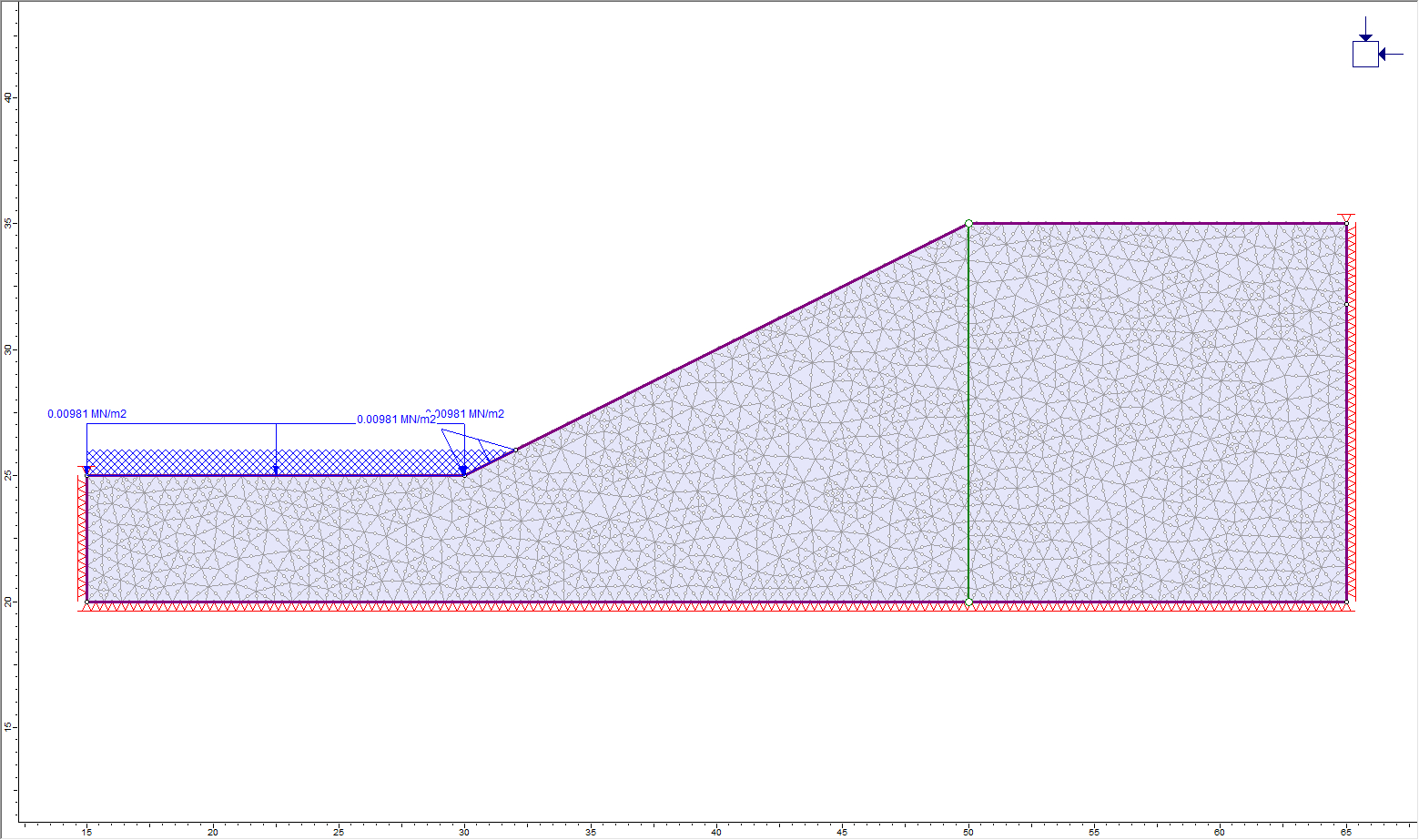

3.0 Compute

1. Select: Analysis > Compute

4.0 Results and Discussion

1. Select: Analysis > Interpret
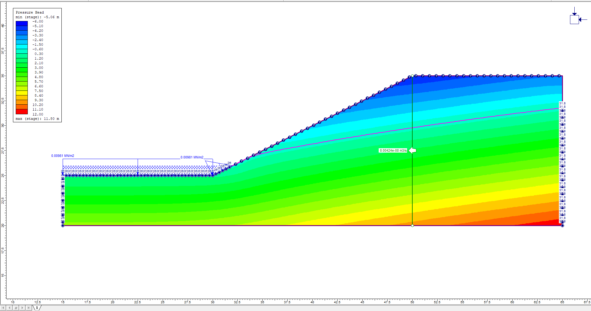
2. Select Seepage > Pressure Head from the data type drop-down menu in the toolbar

The legend in the upper left corner of the view shows the values of the contours. The screen should look as follows:

The contour display can be customized with the Contour Options dialog, which is available in the toolbar, View menu, or right-click menu.

Also, note that by default, the groundwater boundary conditions are displayed (Total Head, etc.).

Display of Total Head values can be turned off in the Display Options dialog (select the Groundwater tab, turn off Show BC Values).

4.1 DISCHARGE SECTION

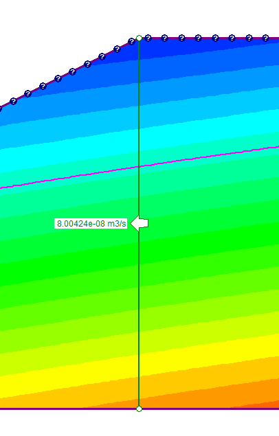
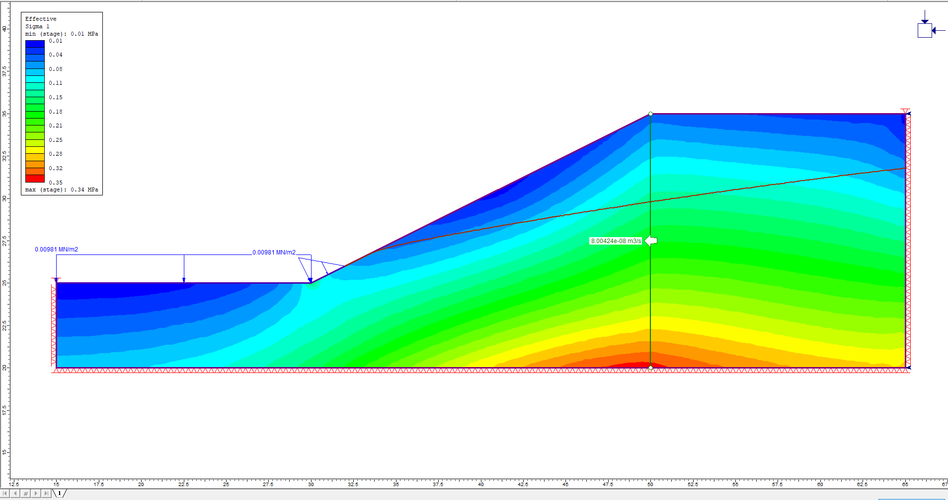
The Discharge Section (the vertical green line segment) displays the steady-state volumetric flow rate of water across the plane of the discharge section.

The flow rate is approximately 8e-08 m3/s across the discharge section in the direction indicated by the arrow:

The display of Discharge Sections can be turned on or off in the Display Options dialog or the toolbar. Right-click on the discharge section and select Hide All Discharge Sections to hide the discharge section.

4.2 WATER TABLE

The pink line on the model indicates the location of the Pressure Head = 0 contour boundary.

By definition, a Water Table is defined by the location of the Pressure Head = 0 contour boundary. Therefore, for a slope model like this, this line represents the position of the Water Table (phreatic surface) determined from the finite element analysis.

The display of the Water Table can be turned on or off using the toolbar shortcut, the Display Options dialog, or the right-click shortcut (right-click ON the Water Table and select Hide Water Table).

Notice that the contours of the Pressure Head, above the Water Table, have negative values. The negative pressure head calculated above the water table is commonly referred to as the “matric suction” in the unsaturated zone. This is discussed later in the tutorial.

To view contours of other data (Total Head, Pressure, or Discharge Velocity), simply use the data type drop down list in the toolbar. Select Seepage > Total Head contours.

4.3 FLOW VECTORS

1. Right-click the mouse and select Display Options.
2. Select the Groundwater tab.
3. Toggle ON the Flow Vectors option.
4. Select Done. (Flow Vectors and other Display Options can also be toggled on or off with shortcut buttons in the toolbar.)

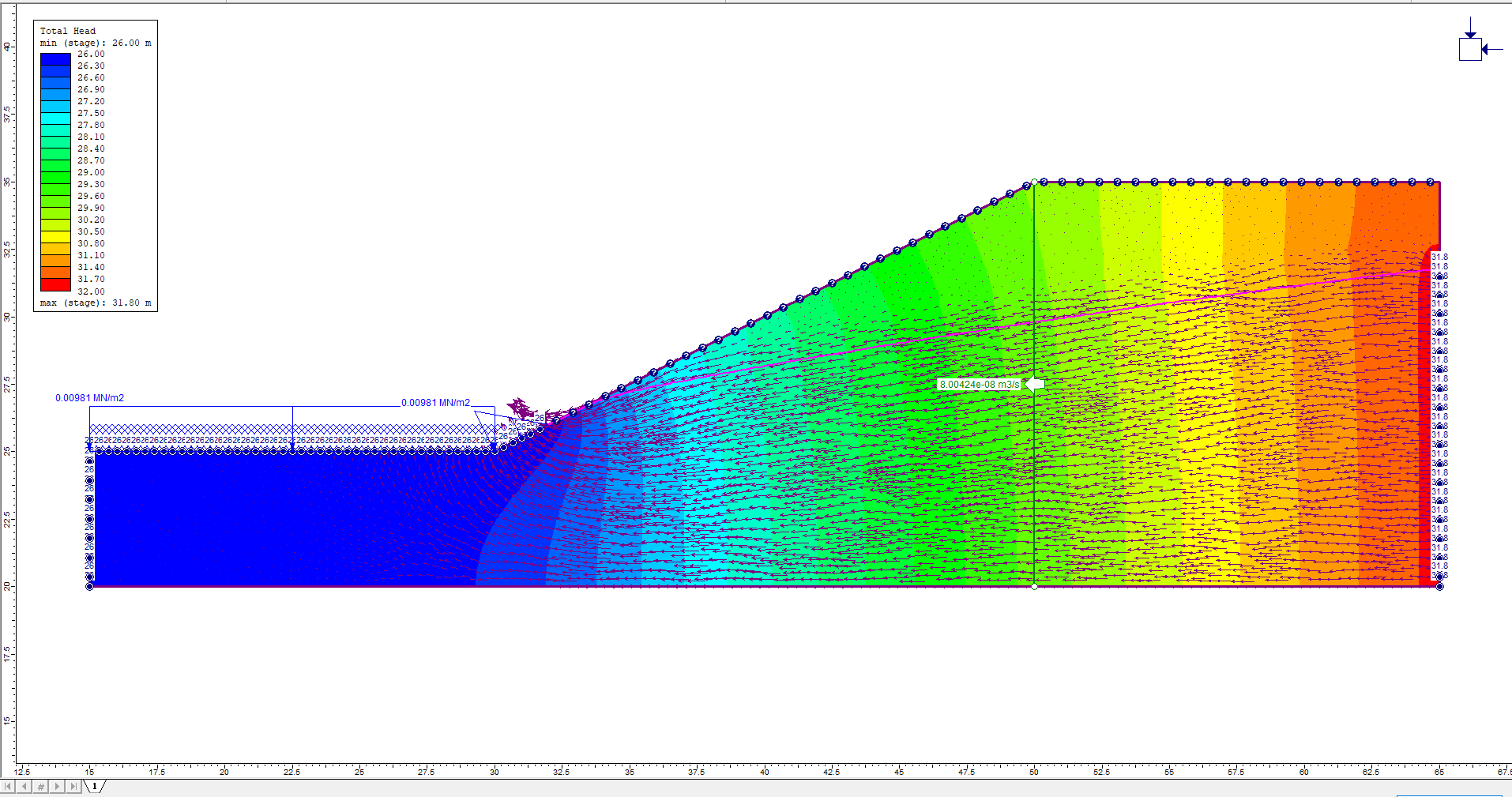
As expected, the direction of the flow vectors corresponds to decreasing values of the total head contours. Notice that there are flow vectors above the water table. This is due to unsaturated flow (i.e. as long as some pore fluid is present, the flow may occur in unsaturated zones above the phreatic surface).

5. Turn off the flow vectors by re-selecting the flow vectors option from the toolbar.
6. Select Total Head contours again.

We can also add Flow Lines to the plot. Flow lines can be added individually, with the Add Flow Line option. Or multiple flow lines can be automatically generated with the Add Multiple Flow Lines option. Let’s do that.

7. Select Add Multiple Flow Lines from the toolbar or the Groundwater menu.
8. Make sure the Snap option is enabled in the Status Bar. If not, right-click the mouse and enable Snap from the popup menu, or click on the word SNAP in the Status Bar.
9. Click the upper right corner of the external boundary, i.e., the vertex at (65,35).
10. Click the lower right corner of the external boundary, i.e., the vertex at (65,20).
11. Right-click and select Done.
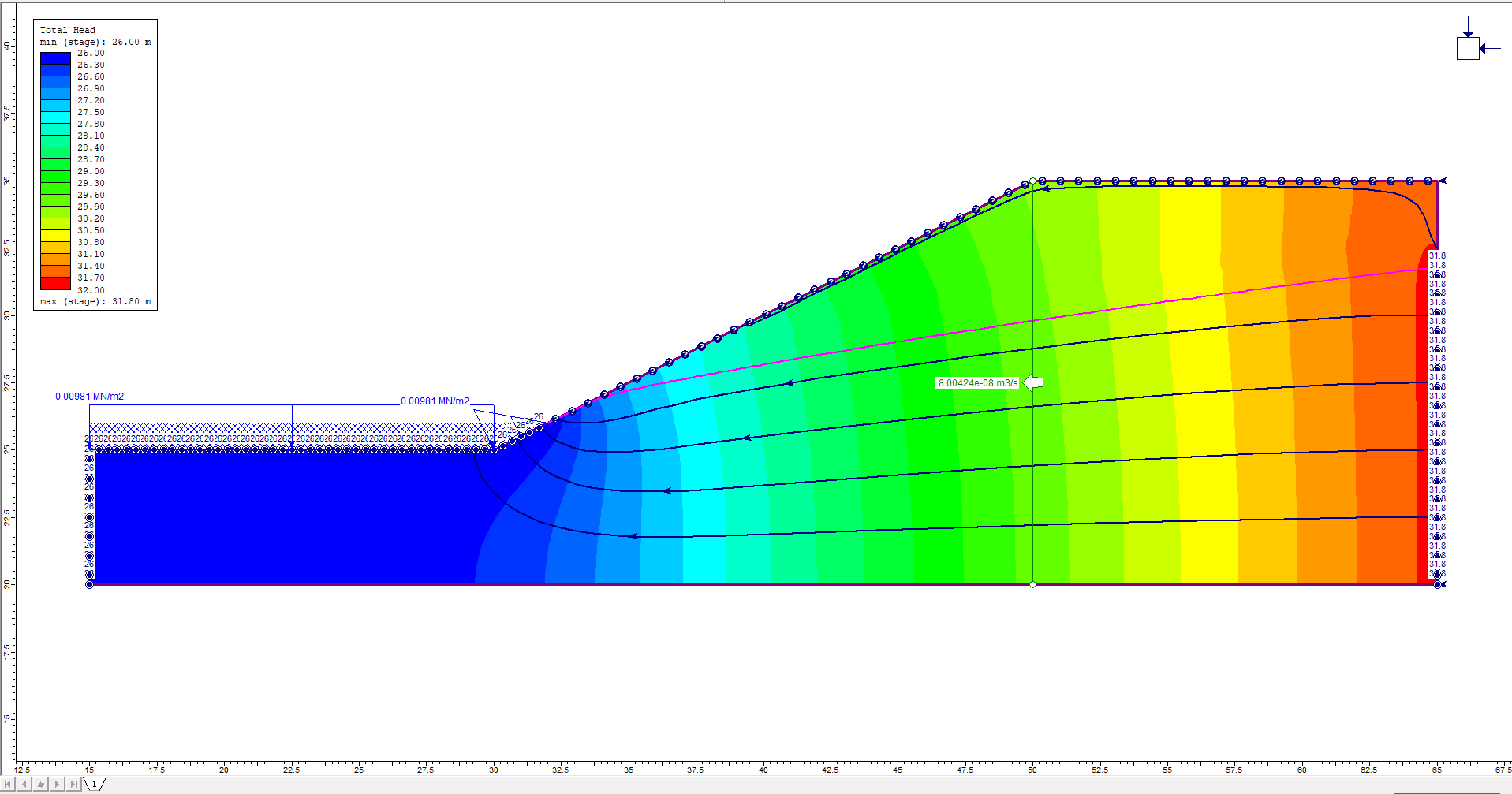
12. You will then see the Flow Line Options dialog. Enter a value of 7 and select OK.
    

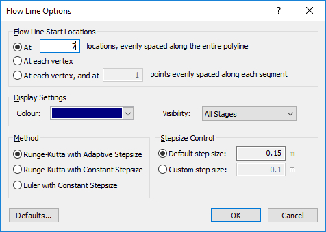
The generation of the flow lines may take a few seconds. Your screen should look as follows:

Notice that the flow lines are perpendicular to the Total Head contours. (Note: only 5 flow lines are displayed, although we entered a value of 7, because the first and last flow lines are exactly on the boundary, and are not displayed.)

Now delete the flow lines.

13. Select Delete Flow Lines from the toolbar or, right-click and select Delete All, and then select OK in the dialog which appears.

TIP: Flow Lines (and Iso-Lines, discussed in the next section) are saved with the RS2 file when you select the Save option. This will save all drawing tools, Flow Lines and Iso-lines, so that you don’t have to recreate them each time you open a file in Interpret.

4.4 ISO-LINES

An iso-line is a line of constant contour value, displayed on a contour plot.

As previously discussed, the pink line represents the Water Table determined by the groundwater analysis. By definition, the Water Table represents an iso-line of zero pressure head. Let’s verify that the displayed Water Table does in fact represent a line of zero pressure (P = 0 iso-line), by adding an iso-line to the plot.

1. First, make sure you select the Pressure Head contours in the data type dropdown menu.
2. Select the Add Iso-Line option from the toolbar, or the Analysis > Iso-Line in the menu.
3. Click on the Water Table line. You will then see the Add Iso-Line dialog.
   
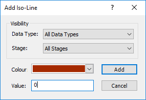
4. The dialog will display the exact value (Pressure Head) of the location at which you clicked. It may not be exactly zero, so enter zero in the dialog, and select the Add button.
5. An Iso-Line of zero pressure head will be added to the model. It overlaps the displayed Water Table exactly, verifying that the Water Table is the P = 0 line.
6. Press Esc or right-click and select Cancel to exit the Add IsoLine option.

4.5 QUERIES

Let’s now add a query to plot the Pressure Head along a vertical profile. The query will consist of a single vertical line segment, from the vertex at the crest of the slope, to the bottom of the external boundary.

1. Select Add Material Query from the toolbar or the Query menu.
2. The Snap option should still be enabled. Click the mouse on the vertex at the crest of the slope, at coordinates (50,35).
3. Enter the coordinates (50,20) in the prompt line, as the second point (or if you have the Ortho Snap option enabled, you can enter this graphically).
4. Right-click and select Done, or press Enter. You will see the following dialog:
   
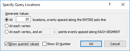
5. For Generate Values, enter "At 20 locations, evenly spaced along the ENTIRE poly-line." Enable the Show Queried Values check box (if it is not already selected). Select OK.
6. The query will be created, as you will see by the vertical line segment and the display of interpolated values at the 20 points along the line segment.
7. Zoom in to the query, so that you can read the values.
8. We can graph these data with the Graph Material Queries option in the Graph menu or the toolbar. Let’s use a shortcut instead.
9. A shortcut to graph data for a single query is to right-click the mouse ON the Query line. Do this now, and select Graph Data from the popup menu.
10. You will see the Graph Query Data dialog. Select the Plot button and the graph will be generated, as shown in the following figure:
    

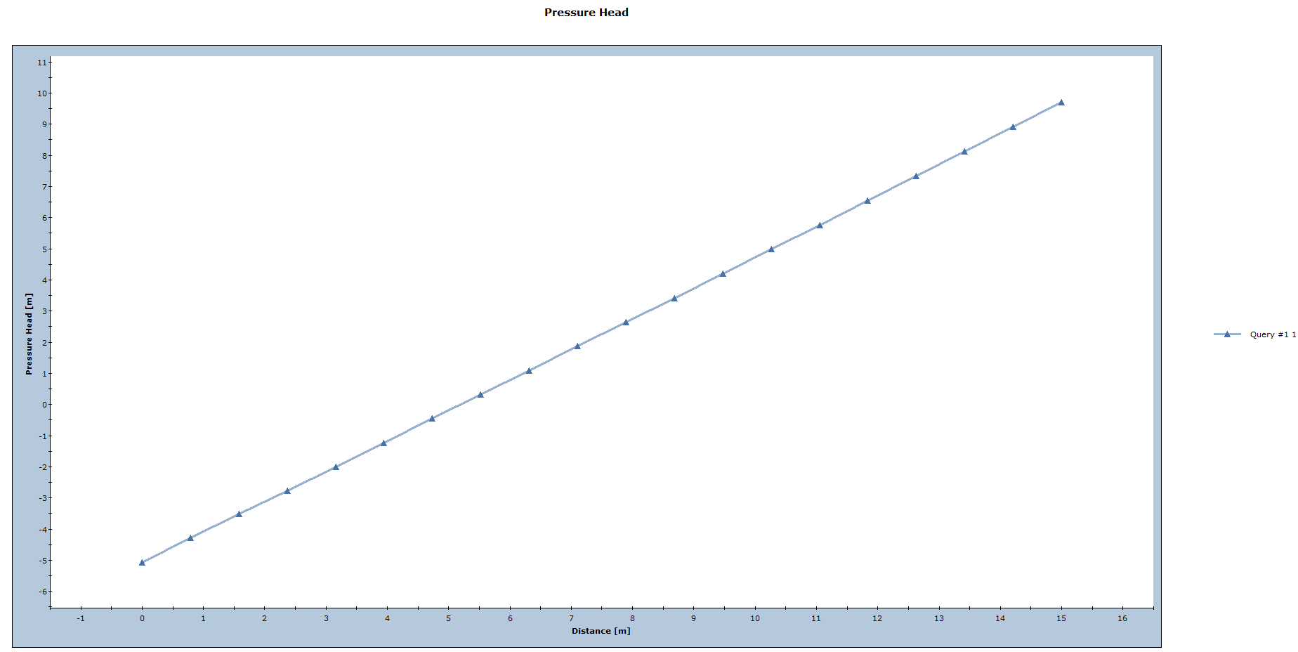
The Query we have created gives us the pressure head along a vertical line from the crest of the slope to the bottom of the external boundary. These data are obtained by interpolation from the Pressure Head contours.

Notice the negative Pressure Head (i.e., matric suction) above the Water Table.

Although we have only used a single line segment to define this Query, in general, a Query can be an arbitrary polyline, with any number of segments, added anywhere on or within the external boundary.

11. Close the graph, and select Zoom All (if you previously zoomed in to read the query values).
12. Delete the Query (right-click on the Query and select Delete Query from the popup menu).

4.6 STRESS ANALYSIS RESULTS

First, let’s hide the groundwater boundary conditions, and display the stress analysis boundary conditions, by selecting the Show Boundary conditions option (available in the toolbar or the Groundwater menu).

The stress analysis boundary conditions are now displayed. This includes the Fixed X, Y restraints on the external boundary, as well as the distributed load due to Ponded Water (represented by the blue arrows applied normal to the boundary at the toe of the slope).

Because we have computed the stress analysis as well as the groundwater seepage analysis, all of the data from both analyses are available for plotting, by selecting a data type from the drop-list in the toolbar.

For example, you can select the following stress analysis results for plotting:

• Principal stresses (Sigma1, Sigma3, SigmaZ)
• Displacements (Total, Horizontal, Vertical)
• Strength Factor
• Effective Stress

The effective stress results in RS2 utilize the pore pressures obtained from the groundwater seepage analysis.

The effective stress results are also used in the failure criterion for each material when computing the Strength Factor and yielding.