New Features in Slide2: Bringing Site Data into Spatial Variability Modelling
- Liam Sy, Geotechnical Software Developer at Rocscience
- Sina Javankhoshdel, Senior Manager - LEM at Rocscience
Real geology doesn't obey global x-y axes, and it certainly doesn't ignore the borehole logs sitting on your desk. Slide2's Spatial Variability feature already allows engineers to represent uncertain soil properties through random fields rather than assigning a single random value to an entire material region. But representing spatial variability is only part of the challenge.
The direction of spatial correlation also matters, particularly where geological structures – such as dipping strata or foliation – have a preferred orientation. And when measurements are available, engineers want those observations to inform the generated field rather than leave it unconstrained at known sample locations.
The latest Slide2 update (v9.045) introduces two capabilities that address these modelling considerations: Anisotropic Spatial Variability, which allows users to control the orientation of spatial correlation, and Conditional Random Fields (CRFs), which incorporate measured site data into field generation. Together, they provide greater flexibility in representing subsurface variability and investigating its implications for slope stability.
Spatial Anisotropy
Spatially variable fields are generated using statistical parameters that define the expected distribution of a property, together with the length over which that property is correlated. Shorter correlation lengths produce more rapidly changing fields, while longer correlation lengths produce smoother zones of similar values.
Until now, spatial correlation has largely been aligned with the model's horizontal and vertical axes. The new anisotropic spatial variability feature removes this restriction, allowing users to specify the direction of spatial correlation.
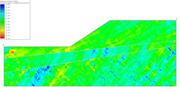
Real geological patterns are not always horizontal or vertical. Layering, depositional structures, foliation, and other site features can create preferred directions along which properties remain similar. The anisotropy implementation follows the directional framework described by Zhu and Zhang (2013). Separation distances are transformed into a rotated and skewed coordinate system before the covariance function is evaluated, allowing the existing covariance formulations to operate on the transformed distances.
Following Zhu & Zhang (2013), two rotational parameters define the orientation of the field:
- Beta (Overall Rotation): Defines the orientation of the principal correlation axis relative to the global framework.
- Eta (Relative Rotation): Adjusts the angle between the primary and secondary correlation axes.
This formulation allows zones of correlation to follow inclined or otherwise directional patterns along specified primary and secondary directions, rather than remaining constrained to the global x-y axes.
These stratigraphical variations can influence the development of failure planes and alter the factor of safety. For example, consider the results of a simple slope analyzed under different anisotropy rotations, as presented by Cheng et al. (2018).
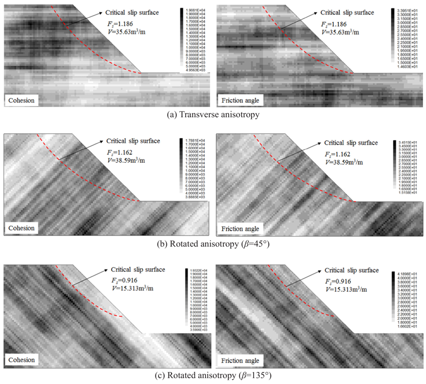
The results show that when the primary correlation axis is parallel to a portion of the failure surface, the factor of safety decreases relative to other configurations.
The underlying field-generation workflow remains unchanged. Existing covariance models and the Local Average Subdivision process can still be used following the coordinate transformation.
Conditional Random Fields
Random fields allow engineers to represent uncertainty in the spatial distribution of material properties. However, an unconditional random field is generated from its prescribed statistical characteristics without requiring it to reproduce specific measurements collected at the site.
This distinction matters when borehole logs or other field investigations provide information about material properties at known locations. Engineers need to represent both the variability implied by the statistical model and the information established by their observations.
Random Fields (CRFs) address this limitation by allowing measured field data, such as borehole observations, to influence the generated spatial pattern, providing a closer representation of the conditions indicated by the available data. Rather than generating a field based solely on its statistical definitions, Slide2 adjusts each realization so that the field responds to the available observations. The following images illustrate the effect of conditioning on a generated field.
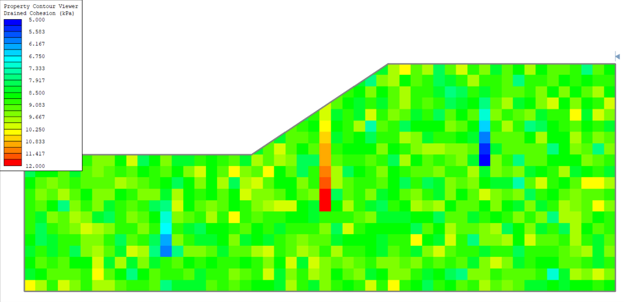
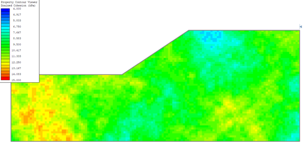
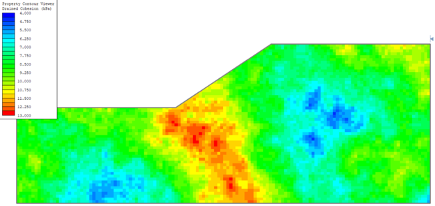
Slide2 performs this conditioning using Conditioning-by-Kriging, a spatial estimation method that determines how strongly each observation should influence a point based on its spatial relationship to that point and to the other observations. In practical terms, nearby and spatially correlated observations have greater influence on the generated field. This allows the field to honour known observations while retaining a representation of the inherent uncertainty between data locations.
Bringing Spatial Variability Closer to Site Conditions
Spatial variability is defined not only by the range of possible material properties, but also by how those properties vary across space and how the available site data inform their distribution. With anisotropic spatial variability and Conditional Random Fields, Slide2 v9.045 extends the ways engineers can represent these relationships in probabilistic slope stability analysis.
The underlying workflow remains unchanged: define the statistical properties, generate spatially varying fields, and investigate their influence on slope stability. What changes is the ability to represent directional correlation and incorporate measured observations within that workflow, providing more flexibility in how subsurface variability is modelled and evaluated.
References
Cheng, Y. M., Li, L., & Chi, S. C. (2018). Risk assessment of slope failure considering the variability in soil properties. Computers and Geotechnics, 103, 139–151.
Fenton, G. A., & Griffiths, D. V. (2008). Risk assessment in geotechnical engineering. John Wiley & Sons.
Zhu, H., & Zhang, L. M. (2013). Characterizing geotechnical anisotropic spatial variations using random field theory. Canadian Geotechnical Journal, 50(7), 723–734.