7 - Automated Region Detection

1.0 Introduction

This tutorial will help you become familiar with automated region detection and area generation on a 3D model in ShapeMetriX’s Analyst tool.

Region Detection is an automated feature for detecting planar patches on a 3D model utilizing user defined resolution and roughness. Detected regions are visualized with a color-coded overlay, can be filtered by geometric and/or orientation attributes and areas can be generated from the detected regions. 

Topics Covered in this Tutorial

• Analysis/Exclusion Zones
• Automated Region Detection
• Filter Detected Regions
• Clustering Preview
• Generate Area

Project Files and Finished Product

The finished product of this tutorial as well as all project materials can be found in the Tutorial 7 – Automated Region Detection.zip  folder.

1.1 Region Detection

The Region Detection feature is closely bonded to the Zone(s) tool. The Zones tool includes Analysis and Exclusion Zones, which will be discussed in detail in Section 3.0 below. If no zones are defined, regions will be detected on the entire 3D model. To apply the Region Detection to specific region(s) or to exclude specific region(s) from Region Detection, be sure to use the Zones tool.

2.0 3D Model Input

If you have not already done so, run the ShapeMetriX (SMX) program by:

1. Double-clicking the SMX icon on the desktop, in your installation folder or by selecting Programs > ShapeMetriX > ShapeMetriX in the Windows Start menu.
2. When the program starts, select Analyst to run the Analyst tool. When Analyst runs, a blank project page opens as shown in the image below.

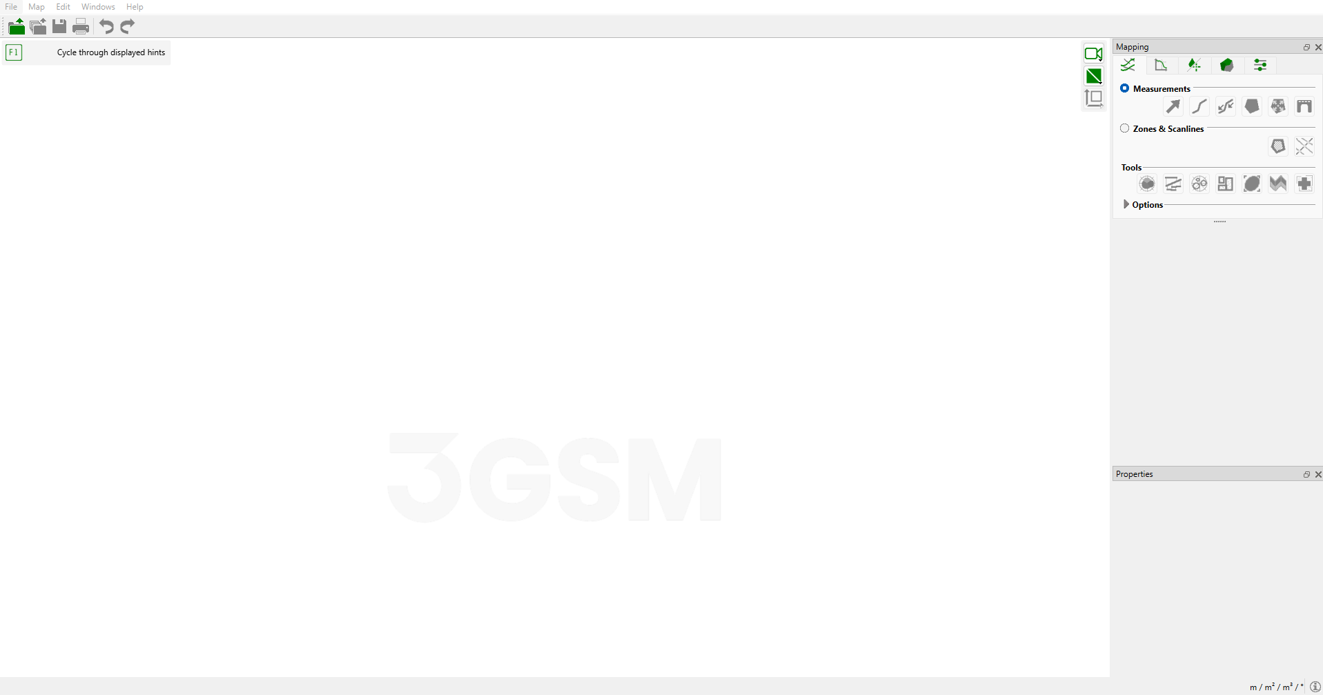
For this tutorial, will use the Bench in Blocky Rock Mass.jm3x file (included in the downloaded Tutorial 7 – Automated Region Detection.zip folder) to demonstrate the Region Detection feature of ShapeMetriX.

1. Select Open 3D Model in the toolbar.
2. Open the Bench in Blocky Rock Mass.jm3x file.

3.0 Analysis/Exclusion Zones 

Analyst includes tools for creating Analysis Zones and Exclusion Zones. Zones are closed polygons drawn by the user on the 3D model. An Analysis Zone selects specific regions for automated Region Detection, while an Exclusion Zone excludes specific regions from automated Region Detection.

Analysis zones are also used to include Areas, Traces and Bridges intersected or surrounded by the polygon, and create subsets of Structure Sets for further Trace Map Analysis. Exclusion zones can also be used to exclude the same from further analysis. 

Multiple analysis and exclusion zones can be outlined on a 3D model. Analysis Zones are outlined with dashed lines whereas Exclusion Zones are outlined with dotted lines in the 3D viewer. Both zones can be managed individually under the Mapping > Structure tab.

3.1 Define Analysis Zone 

To define an Analysis Zone on the 3D model:

1. Select Zones & Scanlines option under Structure tab.
2. Click Zone
3. Mark the border of the zone on the 3D model by clicking the left mouse button. A polygonal line will grow instantaneously.
4. Finish the drawn zone by pressing ENTER or the clicking the Zone button. The defined zone is displayed instantly in the corresponding list under the Structure tab.
5. The defined zone can be assigned as an Analysis Zone or Exclusion Zone using the respective radio buttons under Properties > Zone Type.

In this tutorial, we will define an Analysis Zone on our 3D model as shown below. 

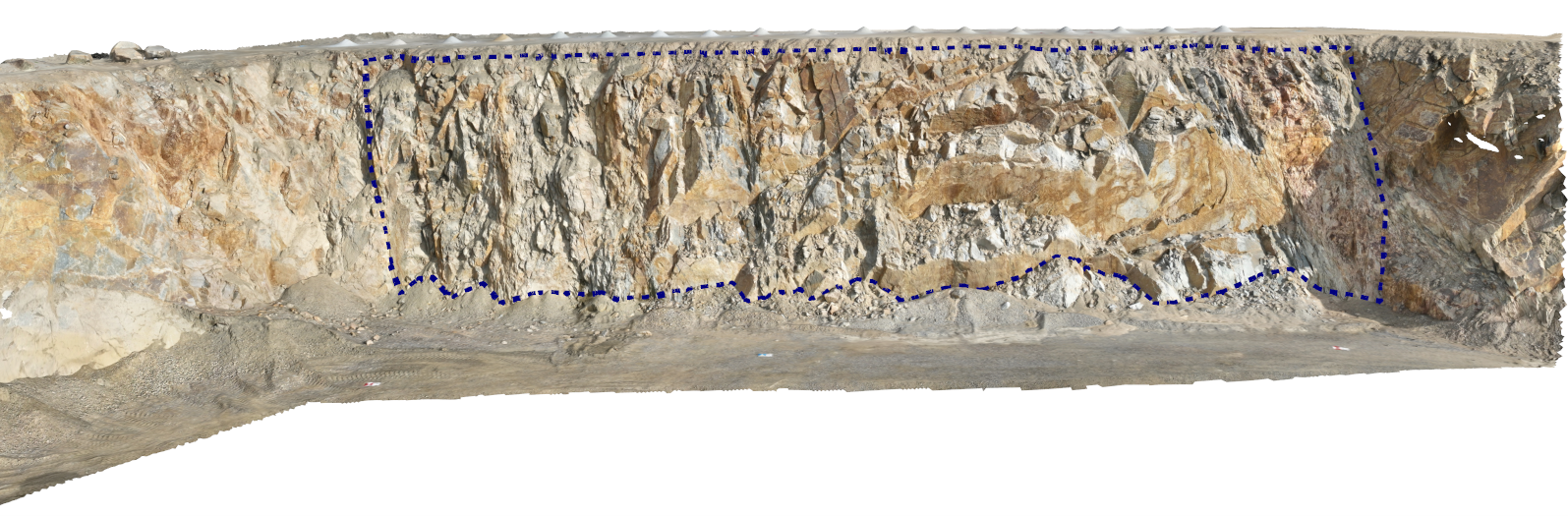
Tip: Zones are outlined with red polygonal lines by default. Zone polyline colors can be changed by right-clicking on a specific zone in the list and selecting Set Colour. Polyline widths can also be changed by adjusting the Polygon Line Width slider under the Settings tab.

4.0 Automated Region Detection

To run the Region Detection for automated detection of planar patches:

1. In the Structures > Tools tab, click  Region Detection
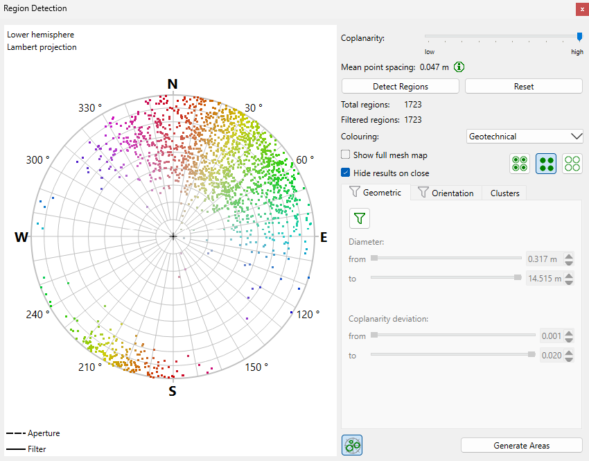
2. The Region Detection dialog will open. Set Coplanarity level to highest using the slider.
3. Select Detect Regions. Detected regions inside the defined analysis zone will automatically be colour-coded on the 3D model. 

The detected regions should be displayed as below.

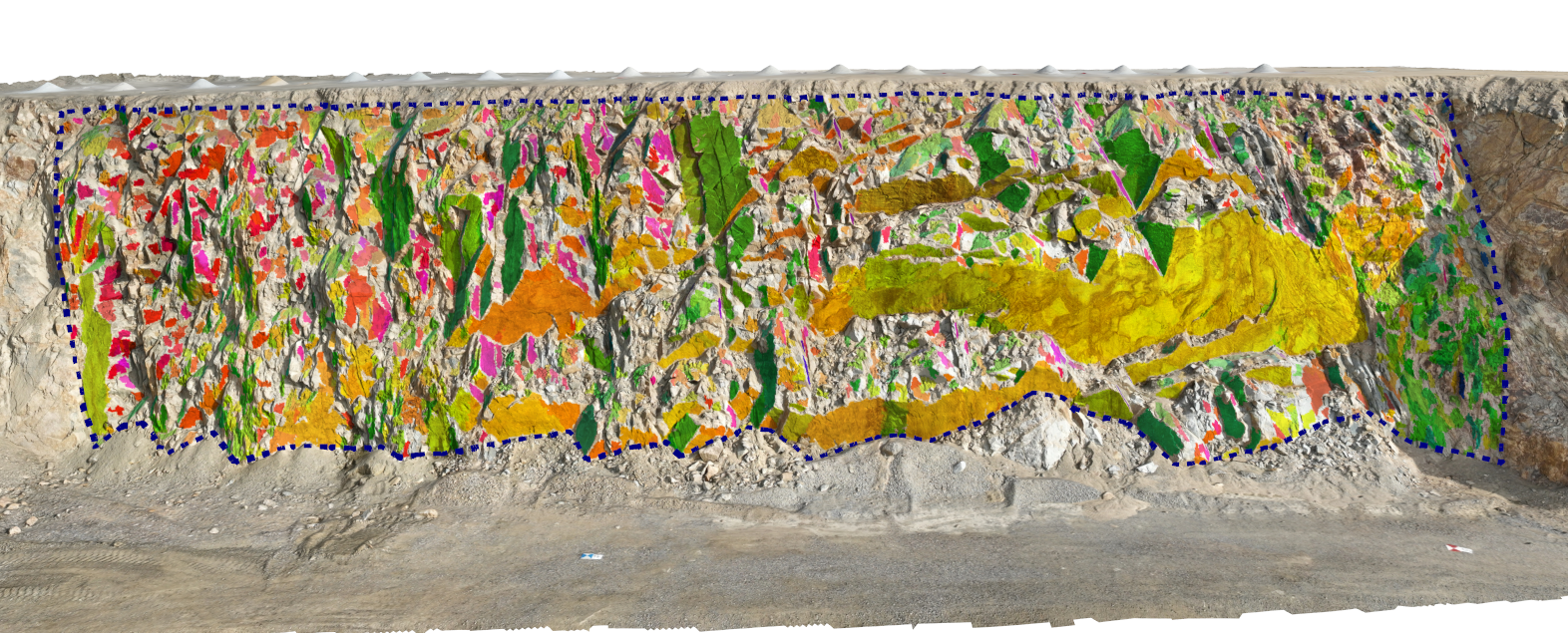
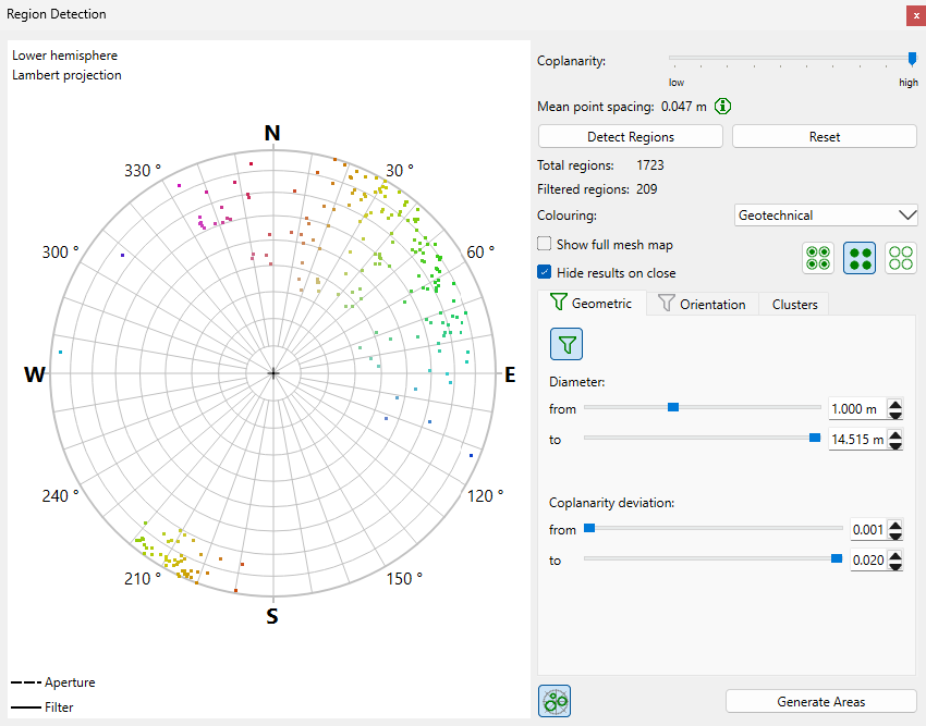
The total number of detected regions is presented and poles of the measured orientations from detected regions are plotted on the stereonet in the Region Detection dialog. 

5.0 Filter Detected Regions 

Detected regions can be filtered according to their geometric and/or orientation attributes using the Geometric and Orientation filter tabs in the Region Detection dialog.

5.1 Geometric Filter 

Geometric filters can be applied to detected regions. In this tutorial, we will apply a size filter to the detected regions. To apply the size filter:

1. Under the Geometric tab, click Filter by Size
2. Set the Diameter from value to 1.0m
3. The defined filter will be applied instantaneously.

Filtered regions will be displayed on the 3D model as below.

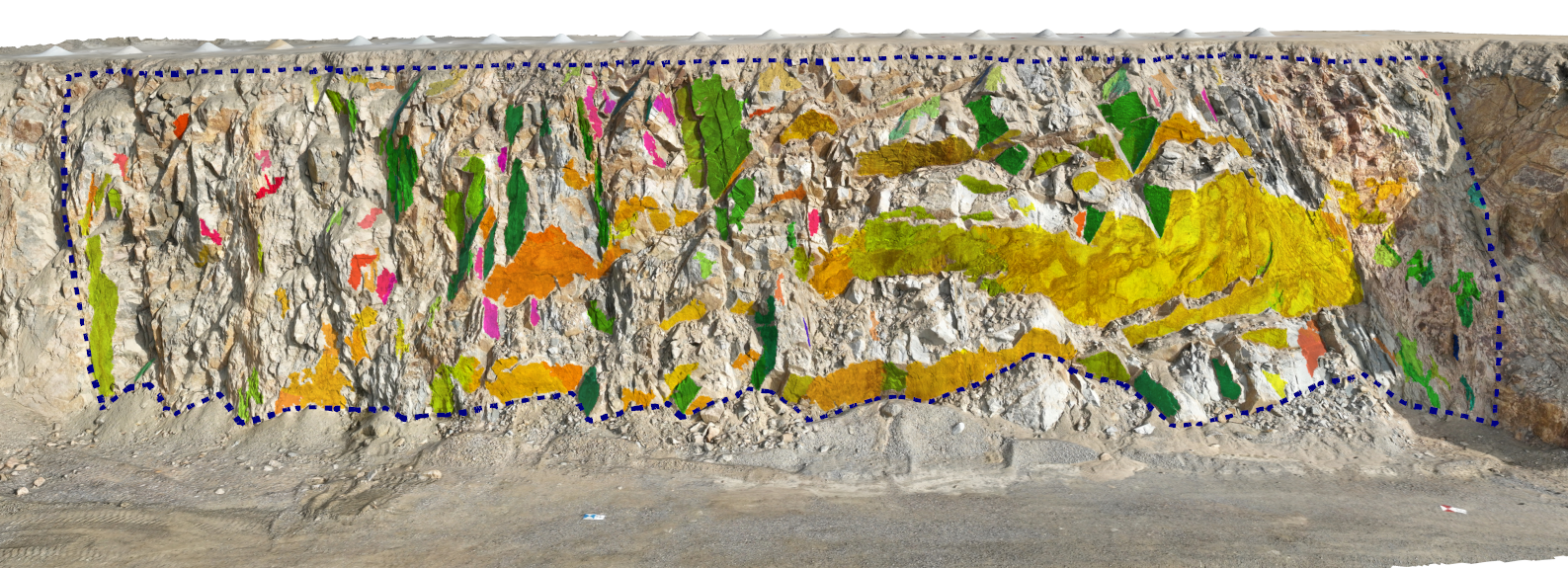
The number of filtered regions is presented in the Region Detection dialog under Total Regions count. The Stereonet plot will also be updated to display the poles of the measured orientations of filtered regions.

5.2 Orientation Filter 

Orientation filters can be applied to detected regions using a Dip/Dip Direction range or by defining a cone. In this tutorial we will apply an orientation filter to the detected regions alongside the size filter. To apply an orientation filter:

1. Under the Orientation tab, click Filter by Orientation
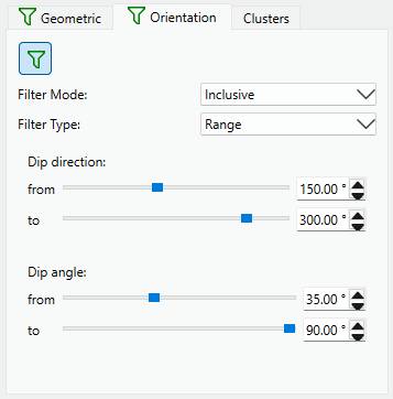
2. Select Filter Mode = Inclusive and Filter Type = Range.

3. Set Dip direction range between 150° - 300° and Dip angle range between 35° - 90°.

   

The defined filter will be applied instantaneously. The filtered regions will be displayed on the 3D model as below.

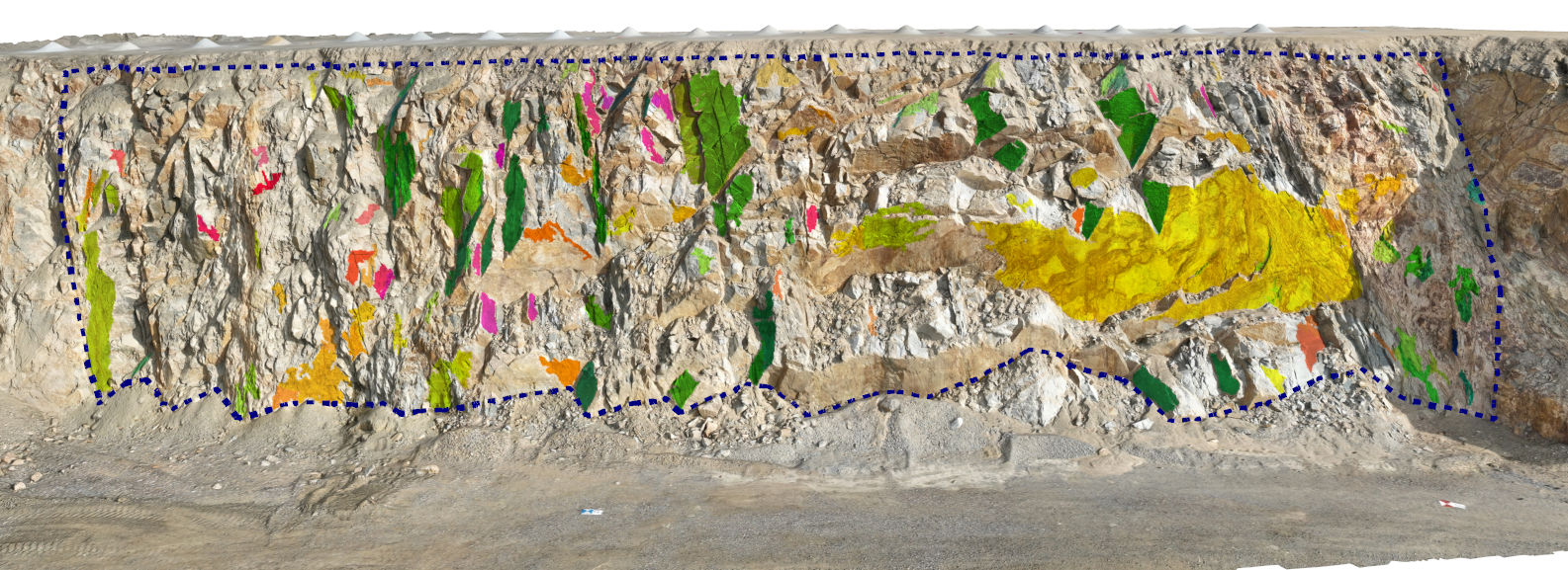
The number of filtered regions is presented in the Region Detection dialog under Total regions count. The Stereonet plot will also be updated to display the poles of the measured orientations of filtered regions.

Let’s change the Filter Type = Cone to apply a filter using a cone. 

1. Set the filter values as follows:
   1. Trend = 30°
   2. Plunge = 20°
   3. Angle = 35°

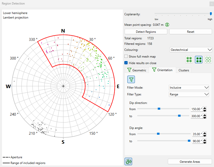
Defined filter will be applied instantaneously. The filtered regions will be displayed on the 3D model as below.

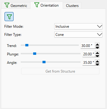
The number of filtered regions is presented in the Region Detection dialog under Total regions count. The Stereonet plot will also be updated to display the poles of the measured orientations of filtered regions.

Tip: Cone axis orientation (trend/plunge) can be set by directly clicking on the stereonet in Region Detection dialog.

Now let’s apply an orientation filter to the detected regions using the orientation of a measured structure. This will enable us to filter regions having similar orientations with the measured structure. 

To get the orientation values from an existing structure and apply them as an orientation filter:

1. Under the Structure tab, ensure the Measurements option is selected.
2. Select Orientation
3. Click on a desired joint surface to get its orientation.

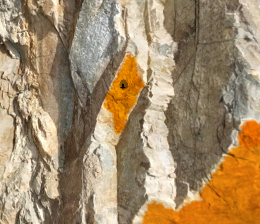
1. Select the Measured Orientation from the map list. 
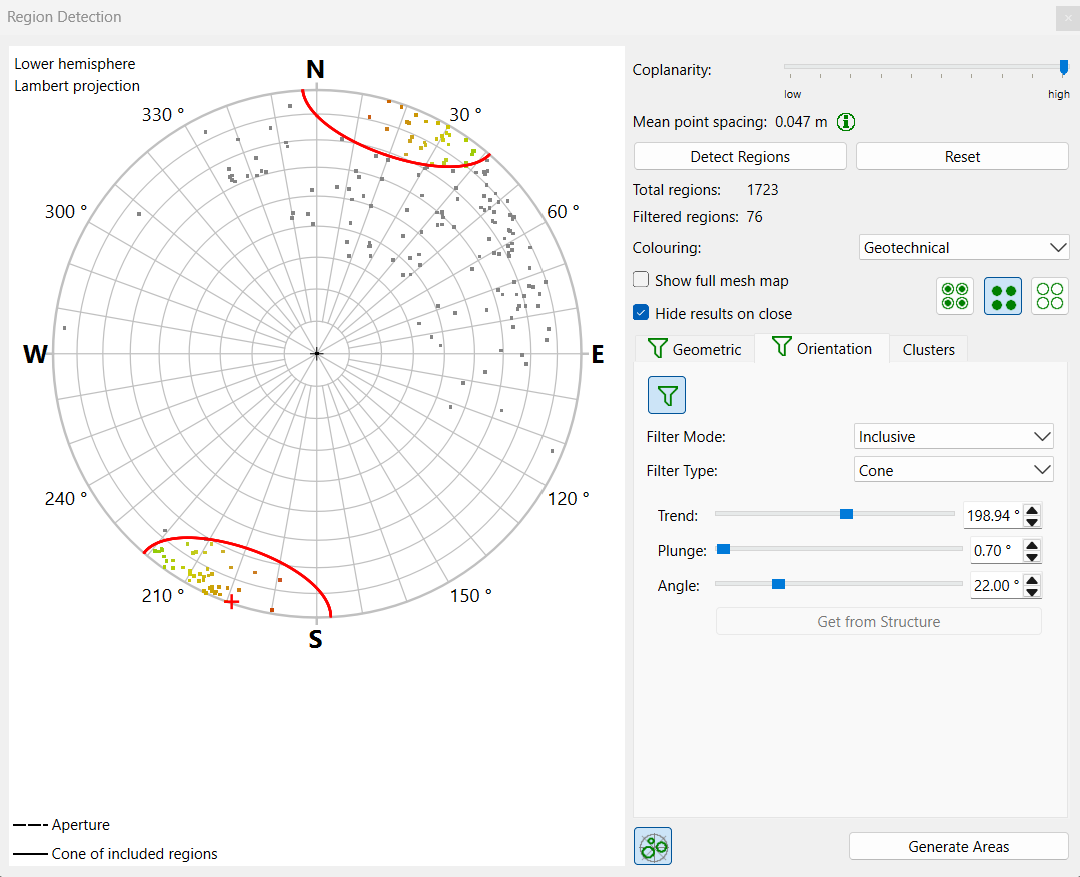
2. In the Region Detection > Orientation tab, click Get from Structure. The Cone’s central axis’ orientation (trend/plunge) is obtained from the measured orientation.
3. Set Angle = 22°.

The defined filter will be applied instantaneously. The filtered regions will be displayed on the 3D model as below.

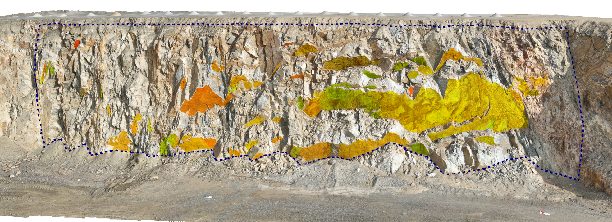
The number of filtered regions is presented in the Region Detection dialog under the Total regions count. The Stereonet plot will also be updated to display the poles of the measured orientations of filtered regions.

6.0 Clustering Preview

The Clusters option in the Region Detection dialog enables a user to group detected (and filtered, if applicable) regions for a preview and generate areas automatically into Structure Sets if clustering applies. 

The Clusters option utilizes non-editable fuzzy K-means algorithm parameter inputs as follows:

• Membership Angle: 90°
• Confidence: 95%
• Weighted by Size: No

If you would like to edit the fuzzy K-means algorithm parameter inputs for a more robust automatic clustering, you should first generate the areas without clustering and then use the Automatic Joint Set Clustering feature. Refer to Tutorial 3 – Geometric Measurement and Structural Mapping for more detailed information on the step-by-step application of the Automatic Joint Set Clustering feature.

To apply a clustering preview in this tutorial:

1. Set Cluster count upper and lower limit as 2 and 6 respectively.
2. Click Cluster Regions.

3. Clusters are determined automatically, and a colour-coded overlay is updated according to cluster colours instantaneously.

   

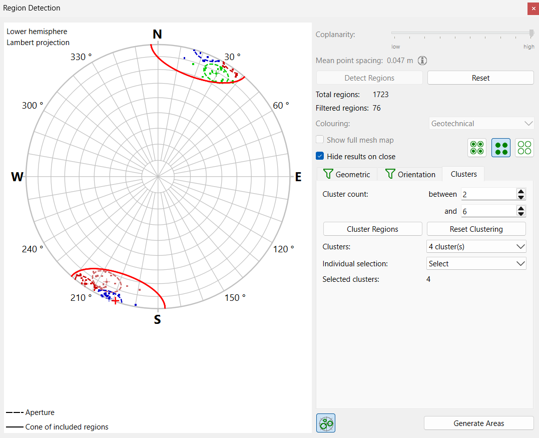
4. Check clustering results. Inspect the results for different clusters counts by selecting the corresponding number of clusters from the pull-down menu.
5. Click Reset Clustering to reset clustering.

Tip: Individual clusters can be excluded from the analysis by deselecting corresponding cluster from the Individual Selection drop down menu.

7.0 Generate Areas

Areas can be automatically generated from the detected (and filtered, if applicable) regions. Since we already applied Geometric and Orientation filters to our initially detected regions, we’ll generate areas from filtered regions.

To generate areas:

1. Click Generate Areas.

Areas will be automatically generated from filtered regions. Generated areas will be displayed on the 3D model as below.

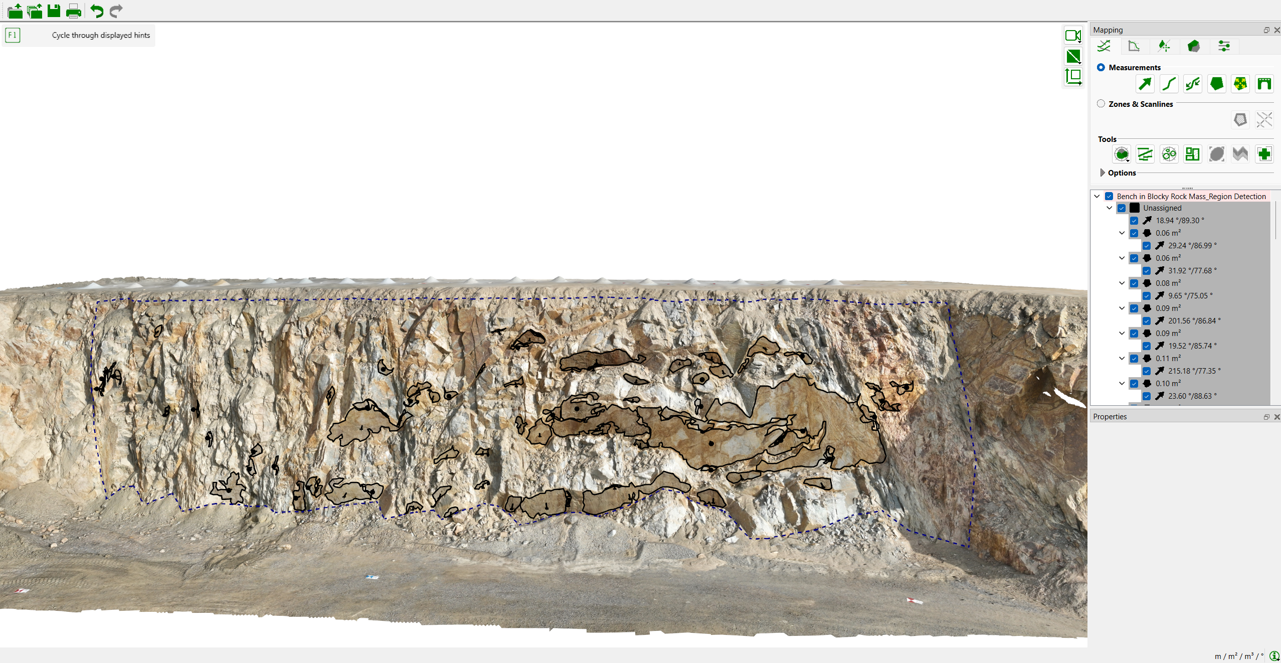
Tip: If clustering isn’t applied to detected regions, areas will be generated under Unassigned joint set by default.

Generated areas are now ready for further analysis.

That concludes the tutorial for Automated Region Detection.