3 - Geometric Measurement and Structural Mapping

1.0 Introduction

Analyst is a convenient tool designed for visualizing and assessing 3D models. It allows users to perform geometric measurements like dip direction and dip angle, areas, distances, point locations etc. directly on a 3D model by marking the appropriate location on the model with the computer mouse. Analyst is specifically designed for analyzing 3D models of rock faces or terrains across various scales, such as tunnel faces, drift faces, caverns, rock slopes, quarries, open-cut mines, laboratory samples, and constructions like dams.

This tutorial will help you become familiar with performing geometric measurements and structural mapping on a 3D model in ShapeMetriX’s Analyst tool.

Topics Covered in this Tutorial

• 3D Model Input
• Basic Settings & Tools
• Structural Mapping
• Adding a Scanline
• Automatic Joint Set Clustering
• Trace Map Analysis
• Stereonet Analysis
• Exporting Structural Map

Project Files and Finished Product

The finished product of this tutorial as well as all project materials are located in Tutorial 3 - Geometric Measurement and Structural Mapping.zip.

1.1 Analyst Functions

 Analyst features a fast and detailed visualization of single, multiple and merged 3D models by the measurements of orientations, distances, lineaments, rock bridges (non-persistent elements), coordinates, occurrences (water, single events), partitioning of areas (lithology and homogeneous areas), and many more, which are called Annotation Elements.

In addition, Analyst also includes attributes like grouping measurements into Structure Sets, semi-automatic trace detection, automatic joint set clustering, orientation of areas and traces including stereographic projection and statistics, defining scanlines and mapping regions, lithologic region and homogenous area mapping, etc. to streamline the geological and geotechnical assessment of rock and terrain surfaces.

Once a 3D model is ready, Annotation Elements can be placed directly on the model. These elements are organized into individual groups:

•  Structures – includes orientation, trace, area measurements, analysis zones and scanlines, discontinuity model, trace map and stereonet analysis, clustering, etc.
•  Geometry - includes volume, area, linearity measurements, contour line, cutoff plane, depth colouring, etc. tools. 
•  Occurrences – includes water, punctual and non-punctual occurrences.
•  Area Partitioning – includes lithological region and homogeneous area mapping.

2.0 3D Model Input

If you have not already done so, run the ShapeMetriX (SMX) program by: 

1. Double-clicking the SMX icon on the desktop, in your installation folder or by selecting Programs > ShapeMetriX > ShapeMetriX in the Windows Start menu.
2. When the program starts, select Analyst to run the Analyst tool. When the Analyst tool runs, a blank project page opens as shown in the image below.

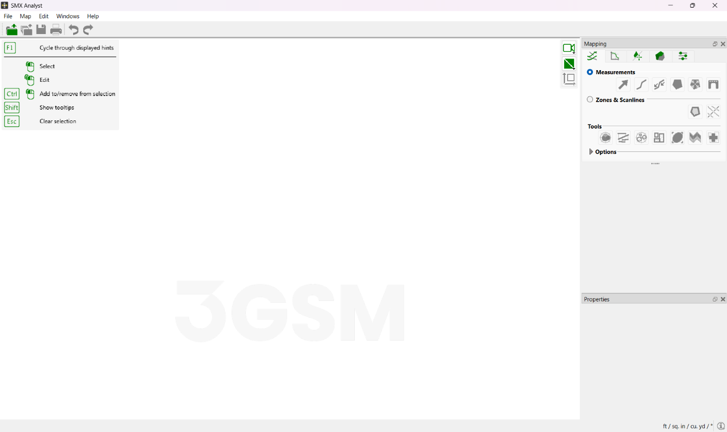
ShapeMetriX comes with several example images and files installed with the program. For this tutorial though, will use the Bench in Blocky Rock Mass.jm3x file included in the downloaded Tutorial 3 - Geometric Measurement and Structural Mapping.zip folder to demonstrate the structural mapping features of ShapeMetriX.

3. Select Open 3D Model
4. Open the Bench in Blocky Rock Mass.jm3x file 

3.0 Basic Settings & Tools

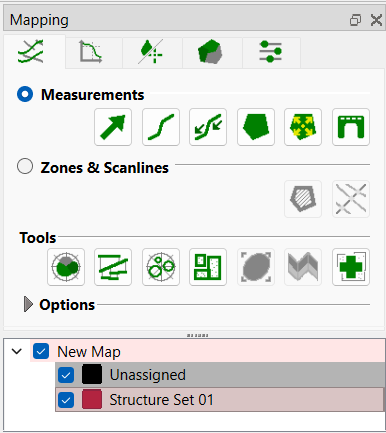
The 3D model is now imported into Analyst. Notice that mapping tools now became visible in the sidebar, and a New Map with Unassigned and Structure Set 1 groups by default has been created under Structures tab. The Properties Pane is also enabled which displays the information of selected Annotation Elements.

The 3D model can be edited, panned, zoomed in and out, oriented, rotated, toggled between projections, etc. using the navigation bar (located in the top right of the 3D model view) or the mouse wheel.  

• Scroll the mouse wheel to zoom in and out.
• Click and hold the mouse wheel to pan the model.

Hint: Analyst toggles between the Edit and Navigate mode by pressing the ESC key. The tool is active when it is blue. 

4.0 Structure Mapping

The Structures tab includes orientation, trace, area measurements, mapping zones and scanlines, discontinuity model, trace map and stereonet analysis, clustering, etc.

4.1 Structure Sets

Structural measurements like orientations, areas, traces, discontinuities, rock bridges are grouped in so-called Structure Sets which can be viewed in the Structure List.

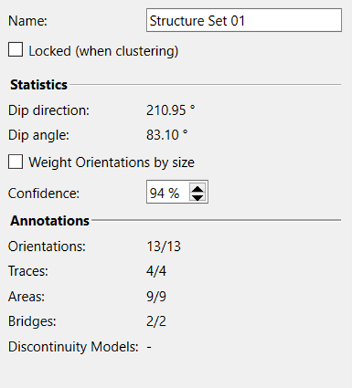
General information of a Structure Set is displayed in the Properties pane when the structure set is selected. Structure set properties include an editable name of the active structure set, the statistics (mean dip direction and dip angle), and number of annotations in the structure set.

4.2 Structure Measurement Types

Structural measurements can be performed by using six measurement tools available in Analyst.

•  Orientation
•  Trace
•  Guided Trace
•  Area
•  Region Grow 
•  Bridge

4.3 Trace Measurements 

Traces are a polygonal line following the object surfaces in 3D space used for annotating linear structures. They are also used to determine the spacing of a Structure Set.

1. Zoom into an arbitrary region in the 3D model that you would like to perform a trace measurement.
2. Select Structure Set 01 in the Structure List.
3. Right click on the Structure Set 01 to change the color to Yellow for improved visibility.
4. Ensure that the Measurements option is active.
5. Select Guided Trace 
6. Mark the start and the end point of the Guided Trace on the 3D model by clicking the left mouse button. A polygonal line surrounded by a cylinder will be visible instantaneously on the 3D model.
7. Adapt the course of the trace by adjusting the cylinder’s width by holding down the SHIFT key and scrolling the mouse wheel. A narrow cylinder results in a straight trace, whereas the trace is allowed to deviate from a straight course by increasing the cylinder’s width.
8. Complete the Guided Trace by pressing the ENTER key.
9. The Trace will automatically add to the Structure List. The length and mean orientation of the trace is provided instantly.
10. Repeat steps 5 – 8 until the desired number of traces are mapped.

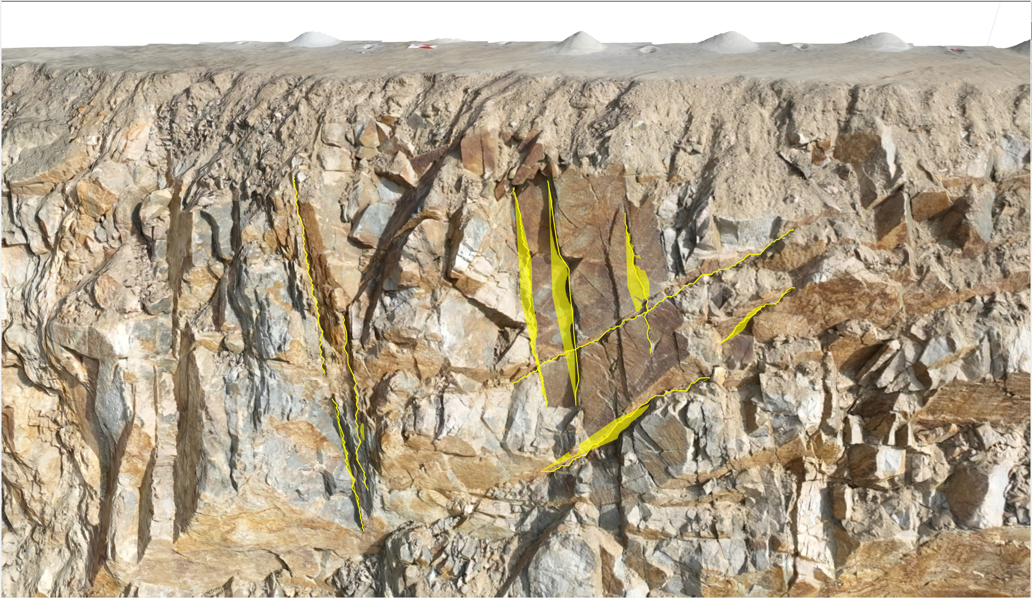
The Length of the trace and its Orientation is added automatically after each trace measurement is completed. The joint plane is indicated by a semi-transparent plane which also delivers the orientation.

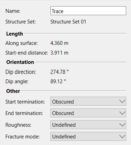
The editable name of the trace, information of which Structure Set the trace measurement belongs to, the length of the trace, the orientation of the joint plane (if determined), the termination index, roughness and fracture mode are provided in the Properties tab when clicked on a specific trace measurement.

Click on the checkboxes next to the area measurements to make them invisible so traces can be clearly visible. Your trace mapping should look as shown below.

4.4 Area Measurements

Area measurements are used for annotating area-based structures (i.e. discontinuity surfaces) or for regions of common geological attributes. 

1. Zoom into an arbitrary region in the 3D model that you would like to perform an area measurement.
2. Select Structure Set 01 in the Structure List.
3. Ensure that Measurements option is active.
4. Select Region Grow
5. Click on an arbitrary point (seed point) on a discontinuity face on the 3D model with the left mouse button.
6. Hold the left mouse button until the desired extension of the Region Grow (i.e. planar patch around the seed point) is obtained by moving the mouse up (increase the extension) or down (decrease the extension) on the 3D model.
7. Release the mouse and an area automatically pops up enclosing a planar patch.
8. Complete the Region Grow by pressing the ENTER key.
9. The Region Grow is automatically shaded and the Orientation (i.e. mean orientation of the surface normal) is added.
10. Repeat steps 4 – 8 until the desired number of discontinuity surfaces are mapped.

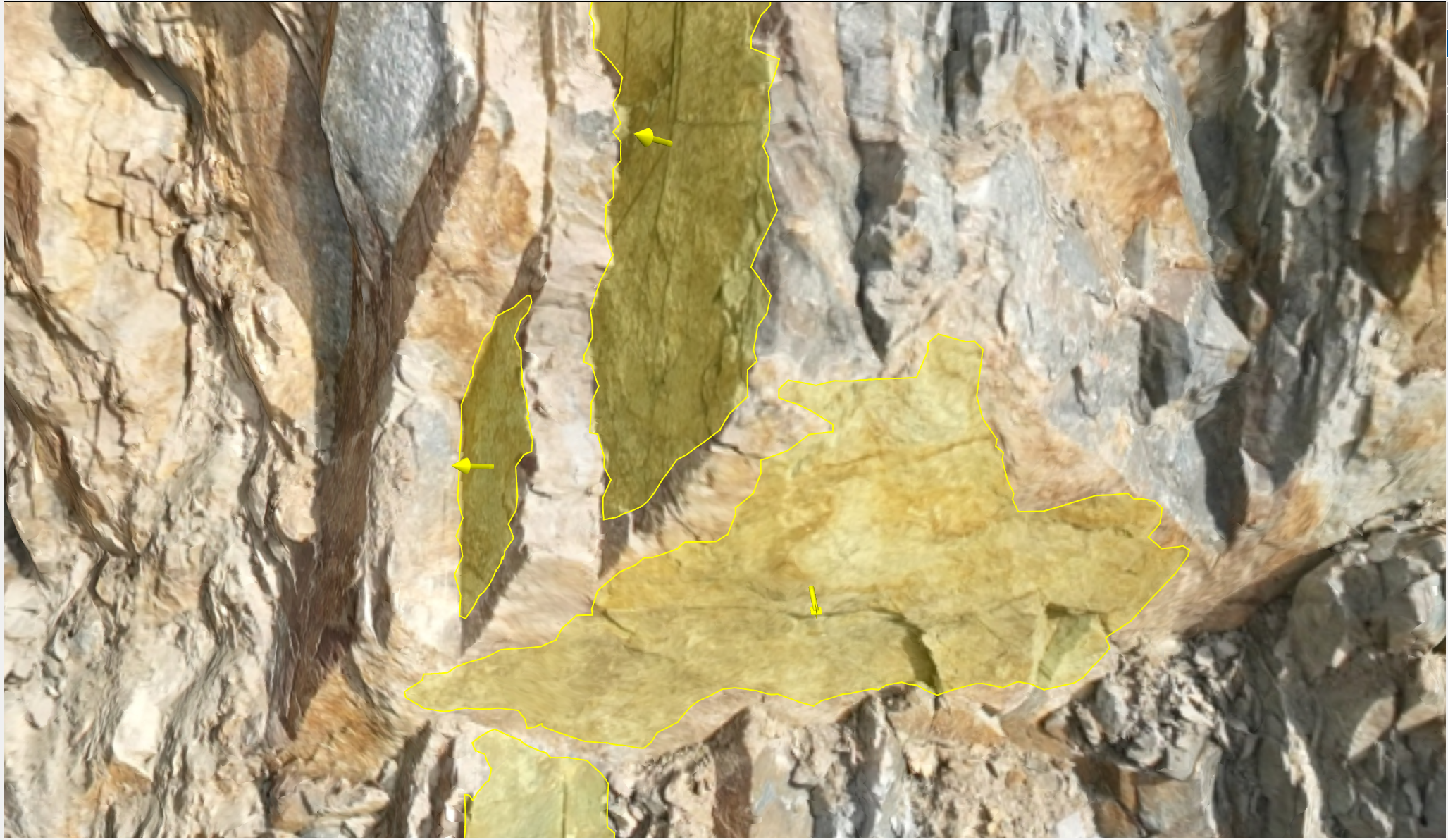
Notice that Arrows and Tails are automatically added to the area measurements after completing each area measurement. The Arrow refers to surface dips towards the observer while Tail indicates an overhanging surface. 

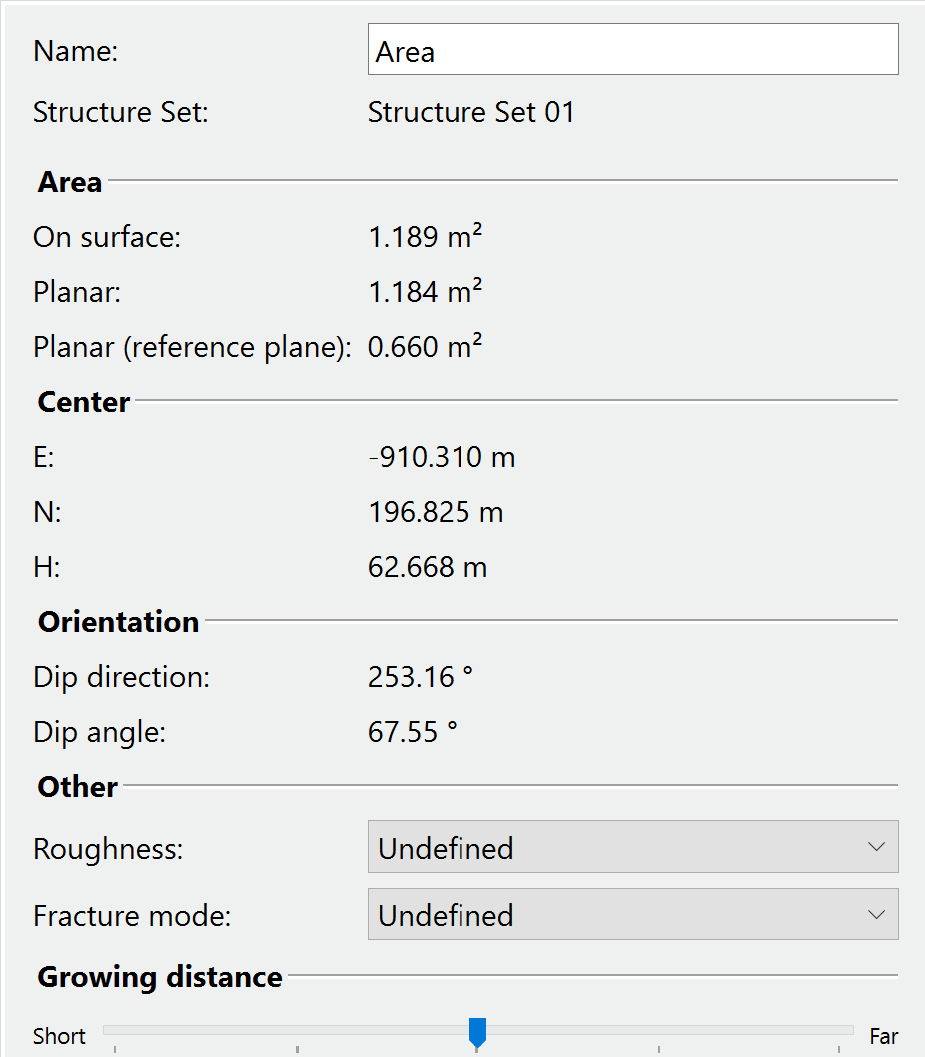
The Size of the area and its Orientation (i.e. mean orientation of the surface normal) is added automatically after each area measurement is completed. The editable name of the area, information of which Structure Set the area measurement belongs to, the size of the area, the orientation of the joint plane (if determined), the exact location (coordinates) of the centroid, roughness and fracture mode of the joint surface and the growing distance are provided in the Properties tab when clicked on a specific area measurement.

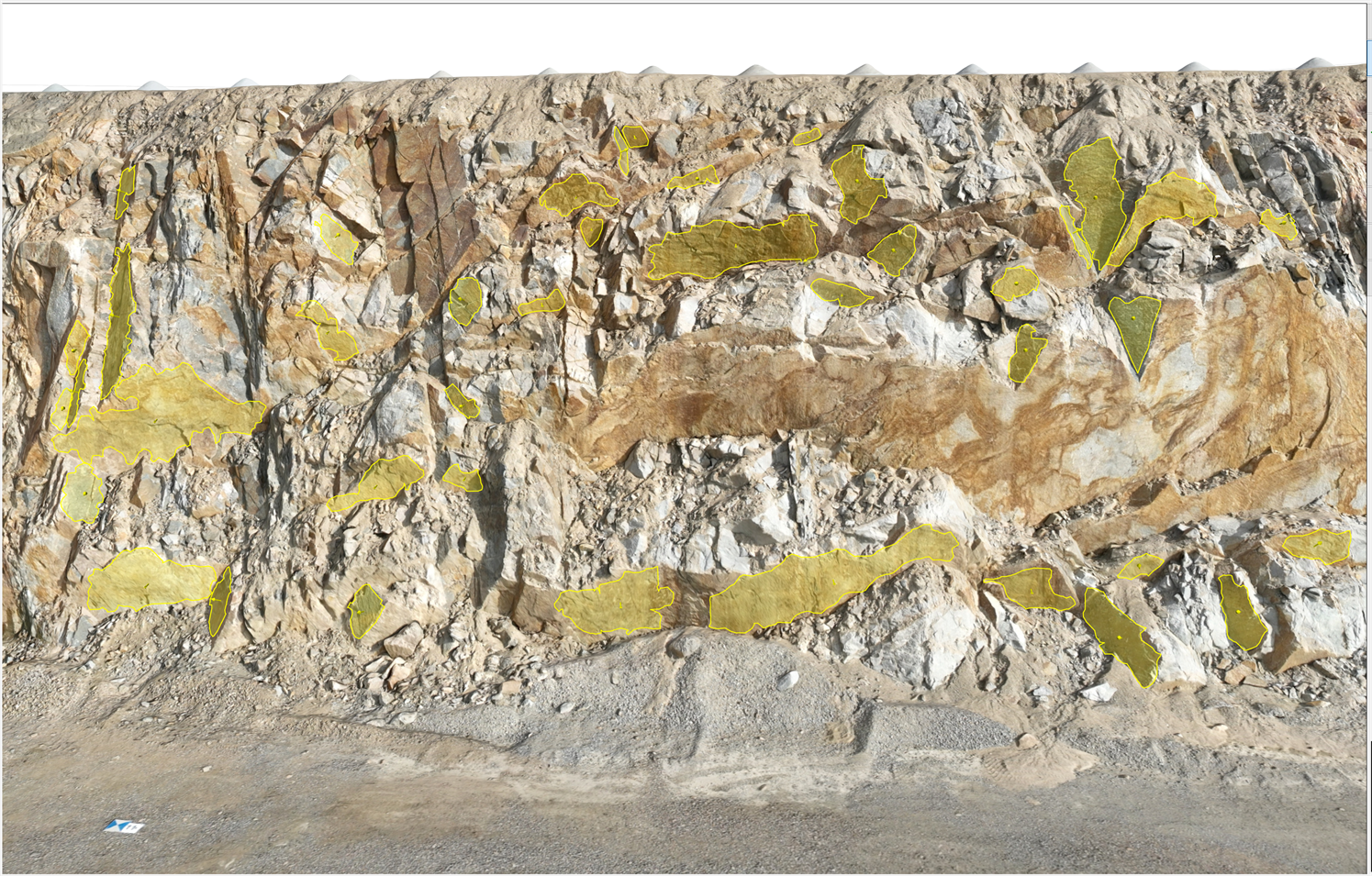
Your discontinuity surface mapping should look as shown below. 

5.0 Discontinuity Models

Discontinuities are used to represent the extent of a fracture. In Analyst, a Discontinuity Model consists of a finite section of a plane confined by a specific planar curve called the Bounding Curve. The plane of this model is determined by the position (given by three coordinates) and the orientation (described by a normal vector, dip direction and dip angle, and an in-plane angle based on the discontinuity's shape) of a Trace and/or Area, or a single Orientation Measurement.

1. Select a Trace or Area from the Structure List.
2. Click on Add Discontinuity Model
3. The orientation of the Discontinuity Model is displayed instantly in the Structure List (i.e. 30.84° / 75.76°).
4. Repeat steps 1 – 2 until the desired number of discontinuity models are mapped (Tip: Discontinuity Models can be assigned all the selected entities in one step by selecting the Traces and/or Areas using CTRL or SHIFT keys).

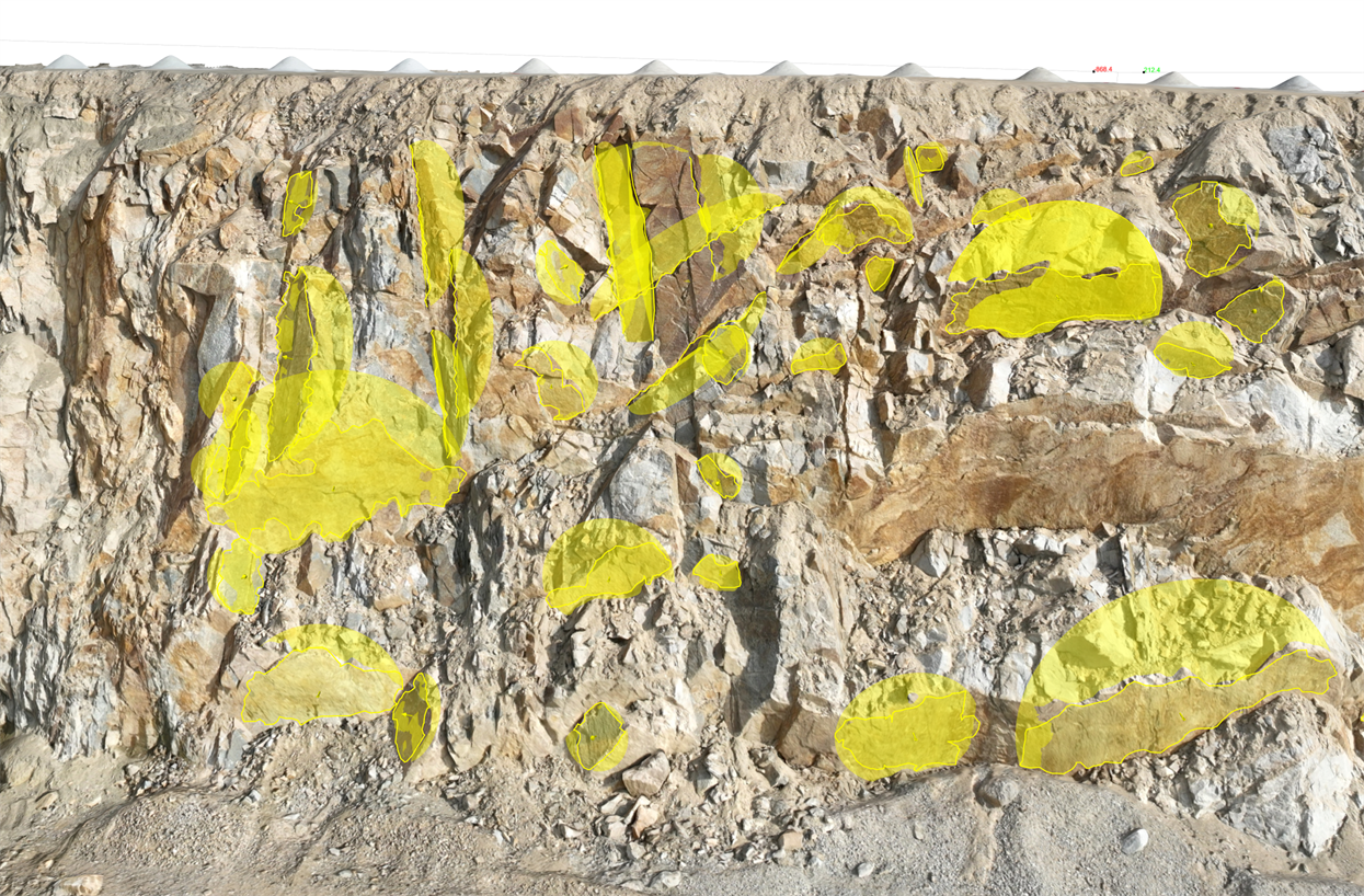
Discontinuity Models can be exported as a .dxf or .csv file by right clicking on a discontinuity model and selecting Export > Export Discontinuity Models as DXF or Export Discontinuity Models as CSV.

6.0 Automatic Joint Set Clustering

Automatic Joint Set Clustering is used to group measured structures automatically into Structure Sets based on joint orientations

Automatic Clustering can be configured using four parameters:

• Cluster Count – defines the number K of clusters. An upper and lower limit is required. Only configurations within the defined cluster count limits will be investigated.
• Membership Angle – defines an angle limit which an Orientation will no longer consider to be included in the cluster beyond the limit.
• Confidence – defines the size of the cone of confidence and affects the statistical cluster separation.
• Weight Orientations by Size – allows to enable weights for each measurement which large structures have more impact on the mean set orientation than small structures.

To perform an automatic joint set clustering:

1. Click on Clustering in the Structure tab toolbar.
2. Set cluster count between 2 and 4.
3. Set membership angle up to 45°.
4. Set confidence to 95%.
5. Click on Cluster to determine the clusters.
6. Review the clustering results for different number of clusters using the Clusters drop down menu.
7. Select number of clusters as three and click Accept Selected Result to confirm the clustering results.

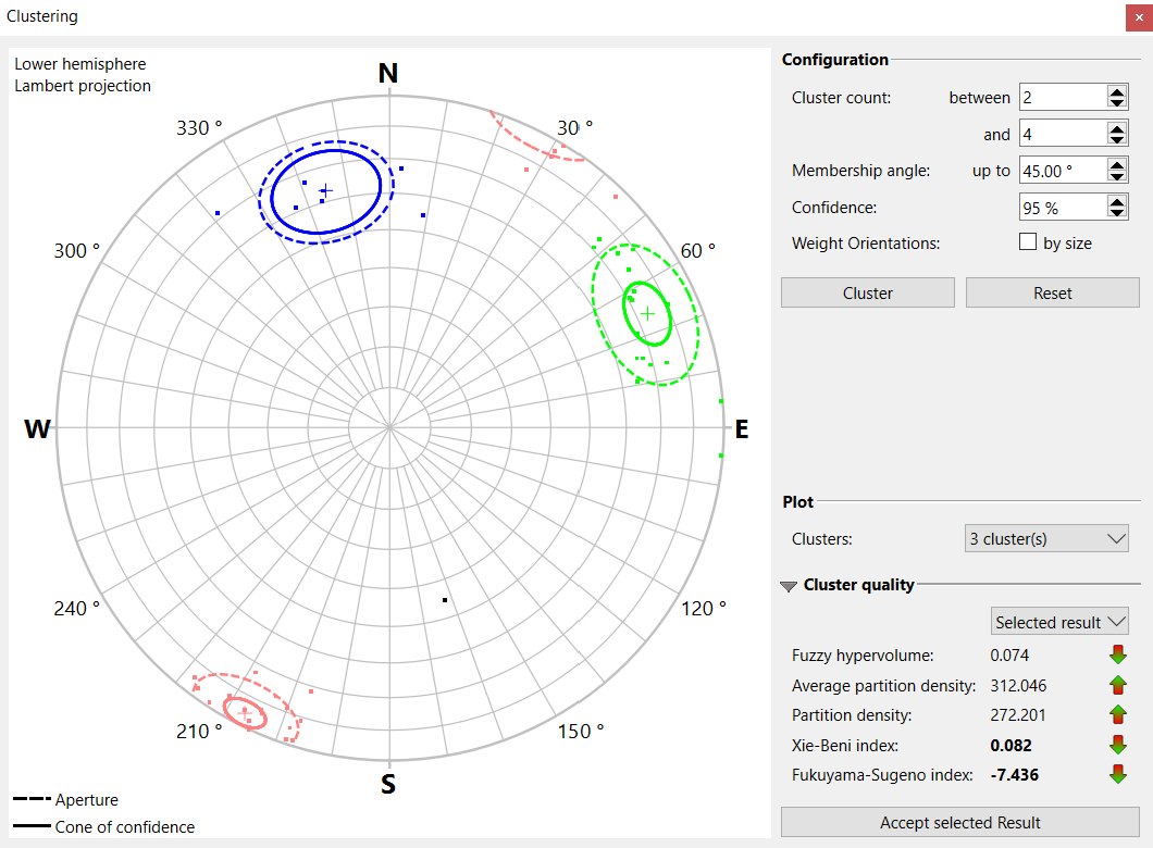
Notice that three structure sets are automatically created in the Structure List and the orientations from the result of the automatic clustering are assigned to each corresponding structure set. The outlier orientations which are filtered and don’t belong to a cluster are assigned to the Unassigned Set.

Click on each Structure Set in the Structure List to see the corresponding mean orientations (set dip direction and dip angle) and number of annotations for each set.

7.0 Trace Map Analysis

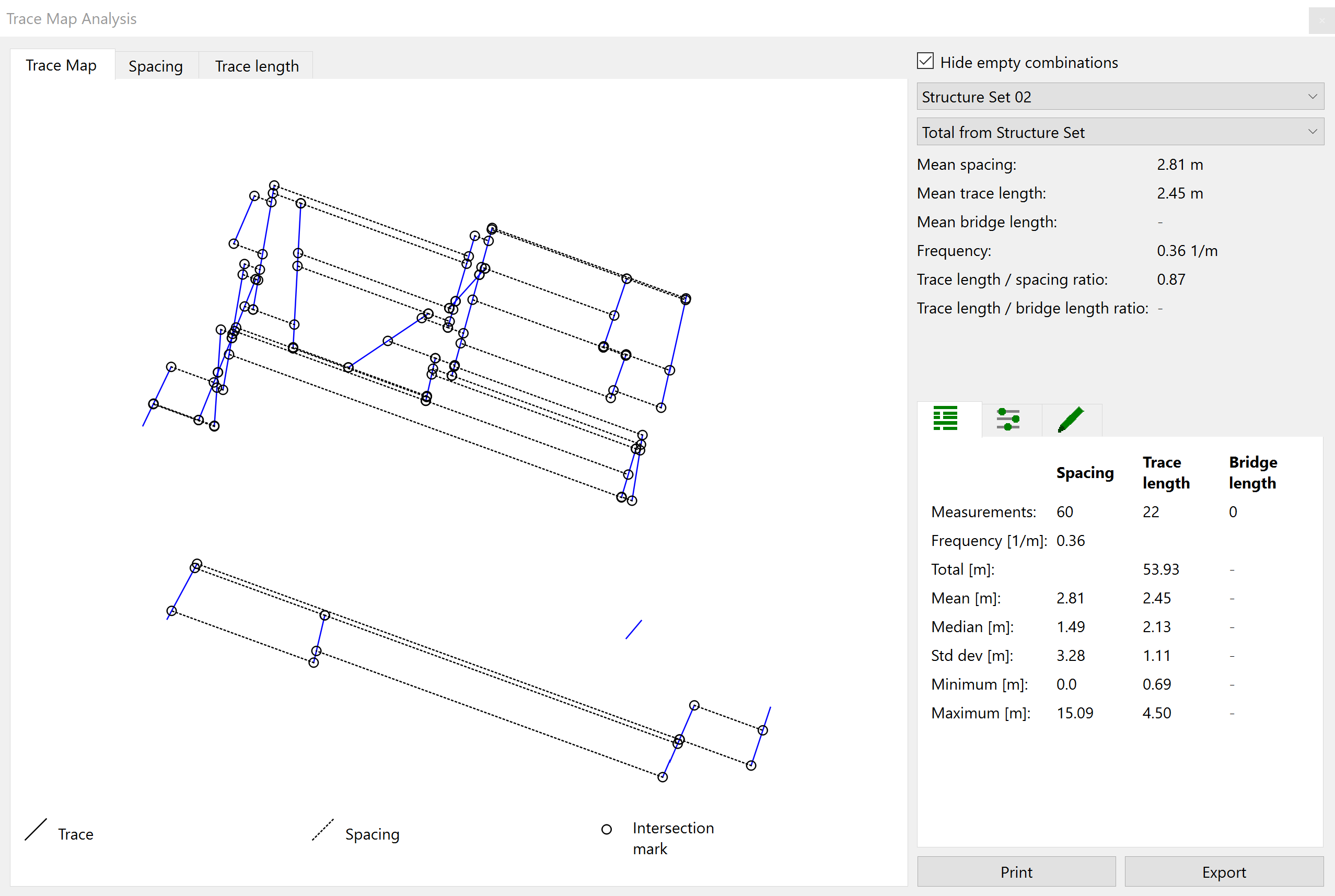
Trace Map Analysis in Analyst is used to visualize data on trace spacing. After opening the Trace Map Analysis dialog, the Projection Plane is displayed in the 3D viewer. Projected Traces appear as non-parallel straight lines in the colour of the Structure Set. Scanlines are outlined as dotted lines whereas the intersection points are indicated by a circle.

To perform a Trace Map Analysis:

1. Click Trace Map Analysis
2. Select the Structure Set you would like to analyze. We will select Structure Set 2  in this example. 

3. Review the spacing calculations and their details.

   

4. Navigate to the Trace Map Configuration tab to edit Projection Plane.
5. In the Projection Plane Tab set:
   1. Rotation = 5.00°

   2. Offset = 1.00 m

      

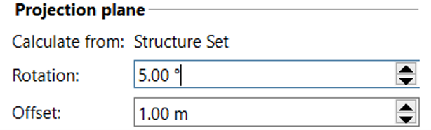
6. Notice that spacing calculations and statistics as well as the projected trace map are updated interactively.
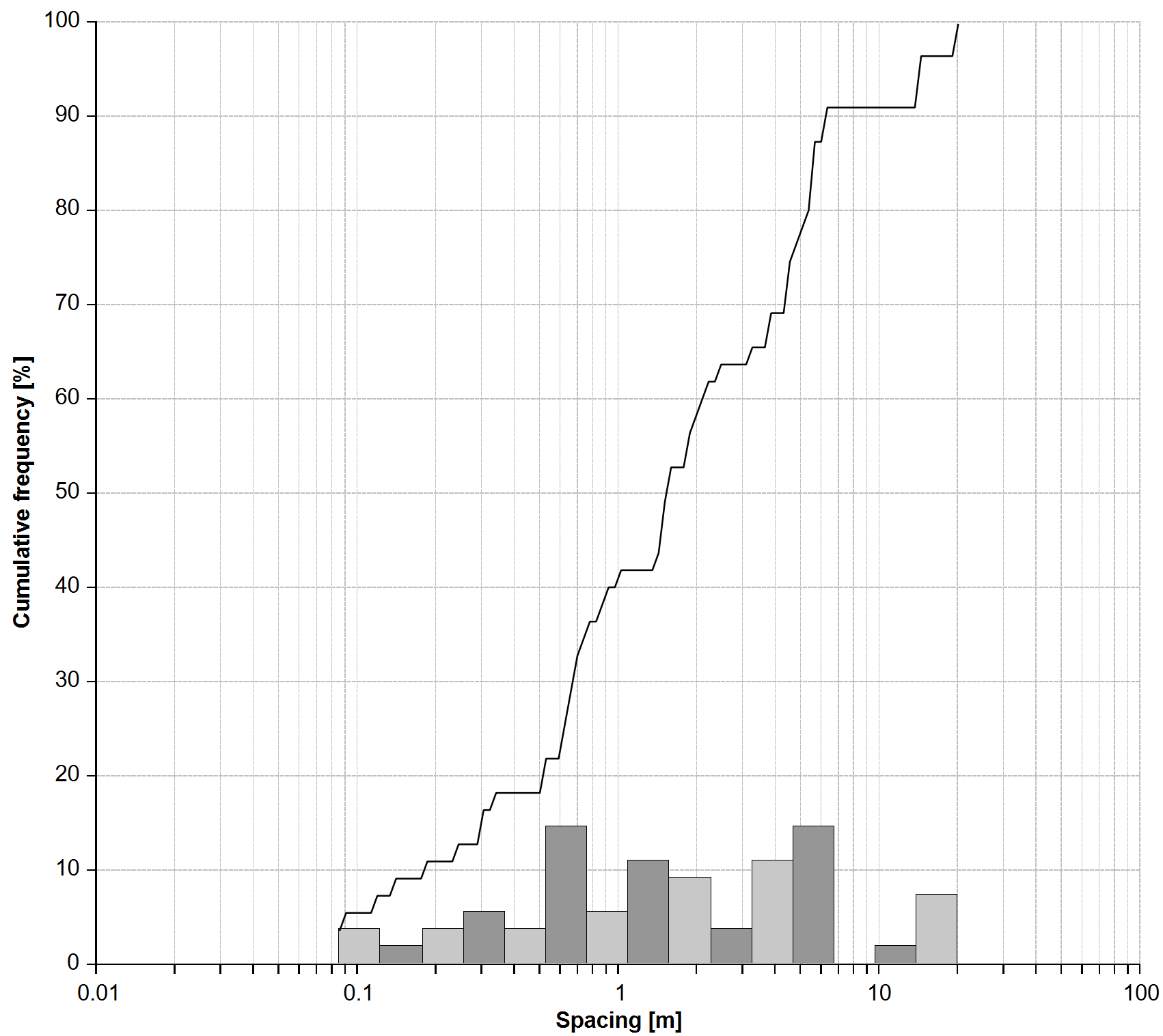
7. Select Spacing and/or Trace Length tabs (at top left of the dialog) to visualize the distribution of spacing and trace length in Histogram Plots. 

8. Select the Plot/Histogram Configuration tab to edit the number of bins as well as scaling which best fits your Histogram Plot.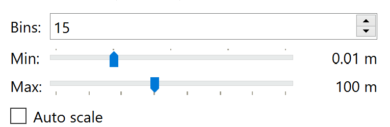

   

9. Your Histogram Plot should look like this.

8.0 Stereonet Analysis

The Stereonet Analysis in Analyst displays the poles of measured orientations for each Structure Set on a hemispherical plot. Alongside this graphical representation, orientation statistics for each Structure Set are also provided.

To perform a Stereonet Analysis:

1. Click Stereonet Analysis

   

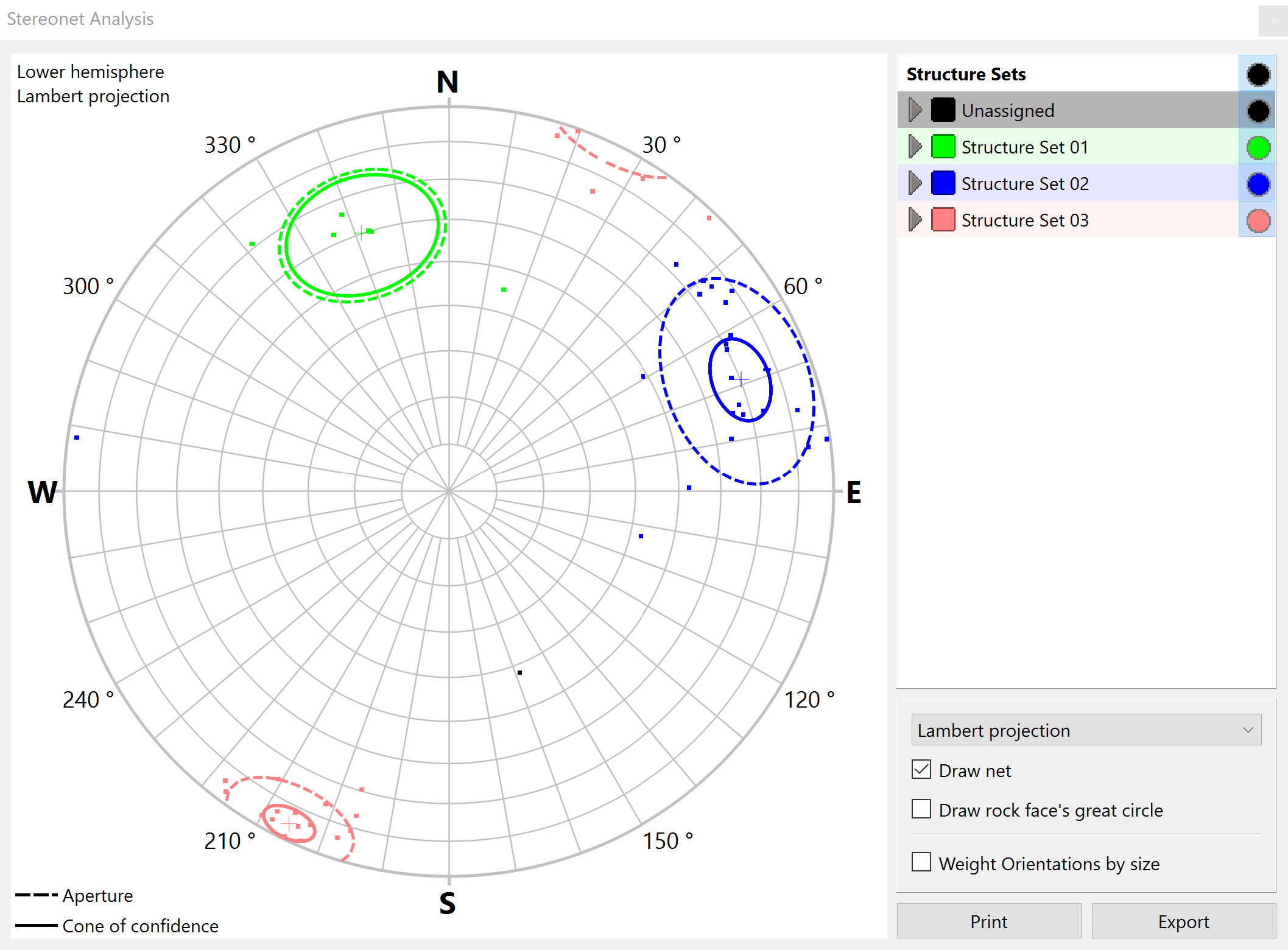
2. Click on the Structure Set you would like to see the corresponding statistics. We will select Structure Set 1 in this example.

   

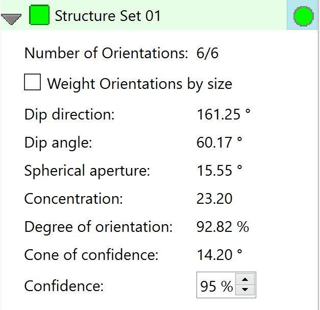
3. Review the statistics for Structure Set 1.
4. Leave all parameters as is and exit the Stereonet Analysis.

9.0 Adding a Scanline

A Scanline is a Structure Tool directly related to geological data evaluation. It is a line along the surface defined by two points identifying the intersections with Traces and Areas, calculating the distances between the intersections and providing statistical data on the joint spacing along the Scanline.

To add a scanline:

1. Ensure that the Zones & Scanlines option is active under the Structure tab.
2. Select  Scanline
3. Mark the start point of the Scanline with a left mouse click.
4. Mark the end point of the Scanline with a left mouse click.
5. Complete adding the Scanline by pressing the ENTER key.

The added scanline will appear as a blue dashed line in the 3D viewer, and it will look as shown below. Notice that the intersection points between the Scanline and Traces/Areas are highlighted when the scanline is selected.

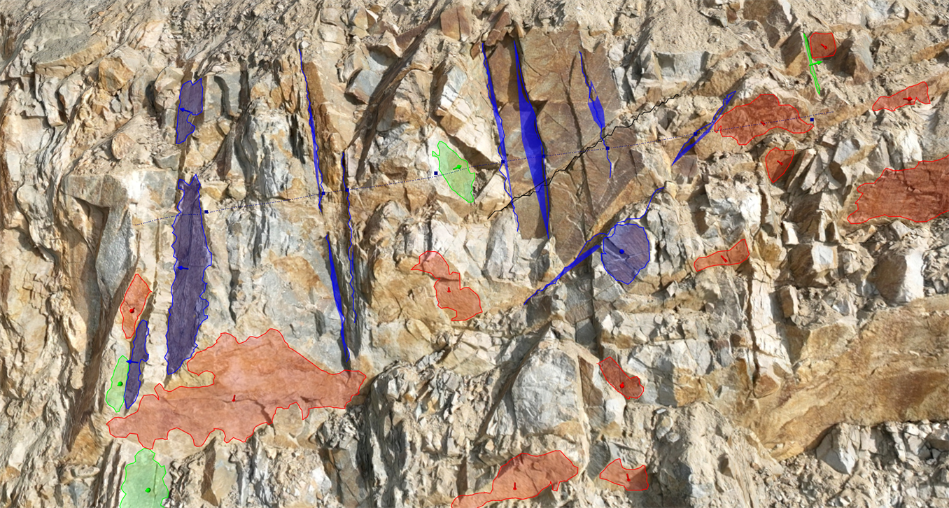
6. Select the added Scanline and change its name to Scanline 1. 
7. Check the Total Spacing statistics for the Scanline and its Trend & Plunge values.
8. Select Structure Set as Structure Set 02 to see the:
   1. Set Spacing Statistics

   2. Normal Set Spacing Statistics

      

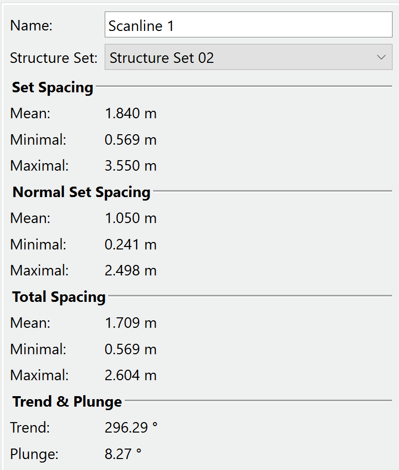
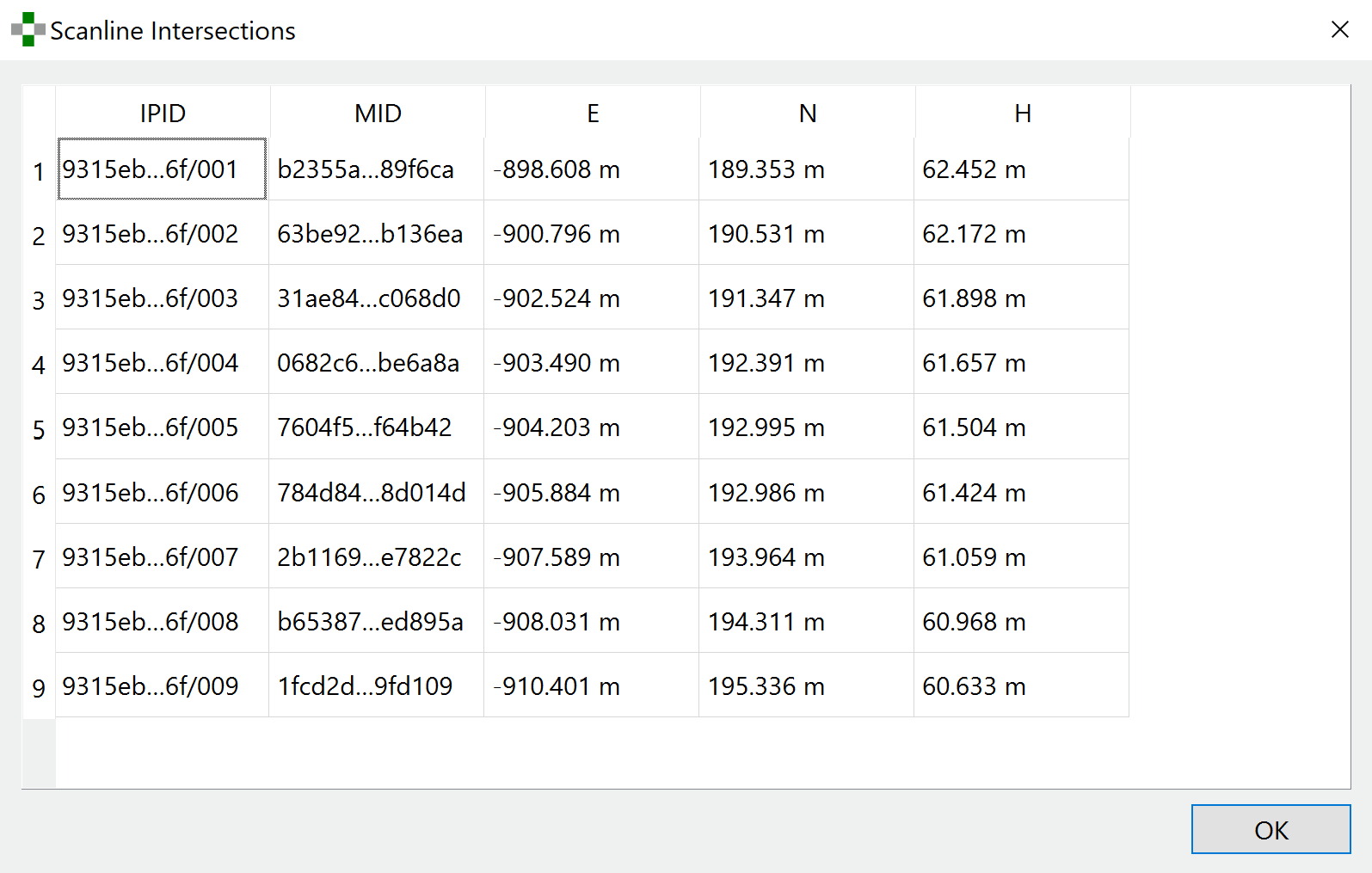
9. Click on Show Intersections in the Properties tab to see the details (ID and exact locations) of each intersection point between the Scanline and Traces/Areas. Scanline details and statistics can be exported as a .csv file by clicking Export.

10.0 Export

Analyst offers various map export options to Dips, .dxf, .obj, .csv, .vrml file formats.

1. Select Map > Export > Export to Dips to export the structural map as a Dips readable file for further Stereonet and Kinematic analysis in Dips.

That concludes the tutorial for Geometric Measurement and Structural Mapping.