1 - Linear Analysis

1.0 Introduction

For this tutorial we introduce users to the basic functions and typical site response analysis flow in the RSSeismic program, while performing a series of Linear Analyses.

We will explore 3 examples of Linear Analyses, looking at both frequency domain and time domain solutions, with undamped and damped soil and rigid and elastic bedrock. Results from these analyses can be compared with standard solutions available in introductory textbooks on this topic. (For example Geotechnical Earthquake Engineering 2^nd Edition by Steven L. Kramer and Jonathan P. Stewart.)

Examples covered in this tutorial:

• Undamped Linear Analysis with Rigid Bedrock
• Undamped Linear Analysis with Elastic Bedrock
• Damped Linear Analysis with Elastic Bedrock

Finished Product:

The finished product of this tutorial can be found in the Tutorial 1 folder. All tutorial files installed with RSSeismic can be accessed by selecting File > Recent Folders > Tutorials Folder from the RSSeismic main menu.

2.0 Example 1a

Undamped Linear Analysis with Rigid Bedrock (Frequency Domain Solution)

2.1 Project Setup

1. Begin by opening the RSSeismic program and selecting New Project

A new project will open, and you will be taken to the Project Setup tab.

The Project Setup option is used to configure the main setup parameters for your RSSeismic project. The Project Setup is where the site response analysis type is selected and is the first step for creating a new project, as some of the settings (for example, the Units System and Analysis Method) determine the inputs and availability of other options.

For this tutorial we will first be selecting a linear frequency-domain analysis. Later in the tutorial we will change the solution type to time-domain for a time-domain linear analysis (Example 1b).

2. Set the Unit System to Metric, stress as kPa.
3. For the Profile Generation, we will be leaving the default: Create Profiles Manually. Since we are only defining one soil profile, Create Multiple Profiles will remain turned off. See the Profiles topic for details on creating multiple profiles.
4. For Analysis Method select Linear.
5. For the Solution Type select Frequency Domain.

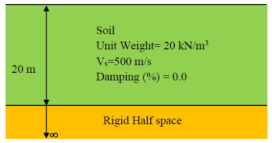
2.2 Profile

1. Select the Profile tab

The Profile tab is used to define the stratigraphy and layers of the soil profile. Users can add/remove layers and define the thickness of each layer. Further soil property details are defined in the Properties tab (which we will address in the next section).

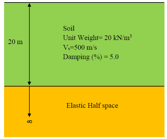
2. In the table on the right, select Layer 1 and enter a Thickness of 20 m.
3. Tick the checkbox for Water table at top of layer. Layer 1 will be selected as it is the only layer.
   
   While in this example the location of the water table does not play a role in the analysis, other more advanced analyses are impacted by the location of the water table.

The Soil profile diagram on the left will update automatically, as will the Soil Profile Metrics below.

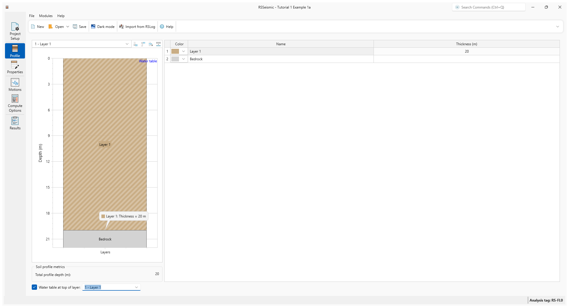
2.3 Properties

1. Select the Properties tab

The Properties tab is used for defining the soil model parameters for your soil profile. Users input their soil properties (unit weight, shear wave velocity, effective vertical stress) for each selected soil layer. Layer 1 will be selected by default. To switch layers, either click on the layer in the soil profile diagram (on the left) or use the drop down list at the top left of the Layer Properties tab.

2. For Layer 1, under Basic Properties enter:
   1. Unit Weight (kN/m³) = 20
   2. Shear Wave Velocity (m/s) = 500
   3. Effective Vertical Stress (kPa) = 101.9
      
3. Select the Soil Model Properties tab.
   1. For Dmin (%) we will leave the default value of 0 for undamped soil.
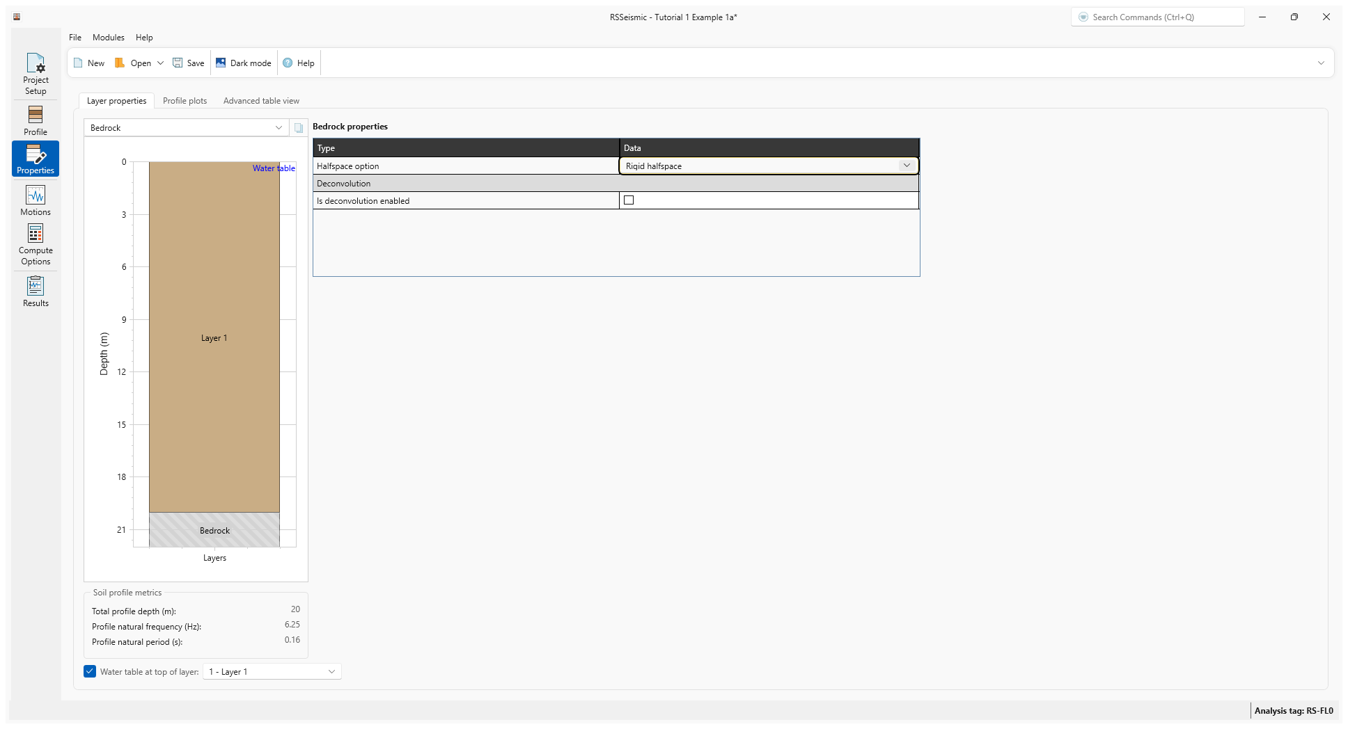
4. Select the Bedrock layer.
5. Note for the Bedrock Properties, the Halfspace option is set to Rigid halfspace. We will leave the default selection.
   

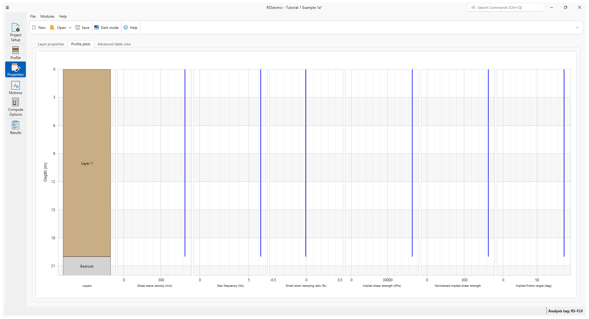
After the definition of basic soil properties and small-strain damping for each soil layer, profile plots such as shear wave velocity, maximum frequency (fmax), and small-strain damping can be viewed in the Profile Plots tab. Other values can be viewed here as well including implied shear strength, normalized implied shear strength and implied friction angle, though they are not relevant for a linear analysis

2.4 Motions

1. Select the Motions tab

The Motions tab is used to select, view and process input motions. RSSeismic has a set of ground motions available within it ground motion library. The motions tab provides the user with a set of tools and capabilities to view and modify ground motions. Users can load their own motions as well. RSSeismic will display acceleration, velocity, displacement and Arias intensity time histories, as well as the response spectrum and Fourier amplitude spectrum for the selected motion.

See the Motions topic for more details on this tab.

For this tutorial, we will select the ChiChi motion.

2. Under Resources/Input Motions, tick the checkbox for ChiChi.
   The time-history (Acceleration, velocity, displacement, Arias and Housner Intensity) and spectral plots (5% damped spectral acceleration) and Fourier Amplitude Spectrum (FAS) of the selected motion can be viewed.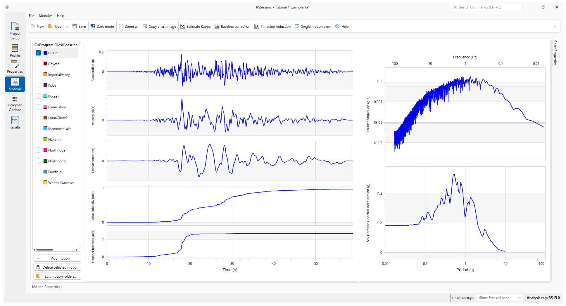
   
3. If you click on Motions Properties in the bottom left of the screen, a pop out table will appear with additional details.
   
4. At this point we should now save the project. Click Save in the toolbar at the top of the screen (or select File > Save Project ) and save this project as Tutorial 1 Example 1a.rsseismicfile.

2.5 Compute

1. Select the Compute Options tab

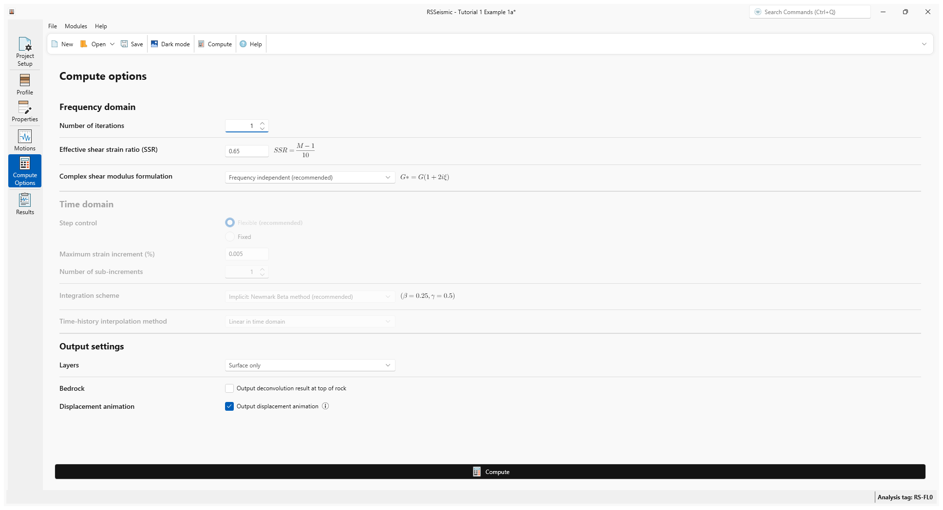
Since we have selected a Frequency Domain solution, only the Frequency Domain options will be available.

2. Under Frequency Domain enter:
   1. Number of iterations = 1
      
      Since the analysis is Linear no iterations are needed.
   2. Effective Shear Strain Ration = 0.65
   3. Complex Shear Modulus Formulation = Frequency Independent (recommended)
3. For Output Settings, leave the default Layers = Surface Only. Output Displacement Animation should also be turned ON by default.
   
4. Click Compute at the bottom of the window.

2.6 Results

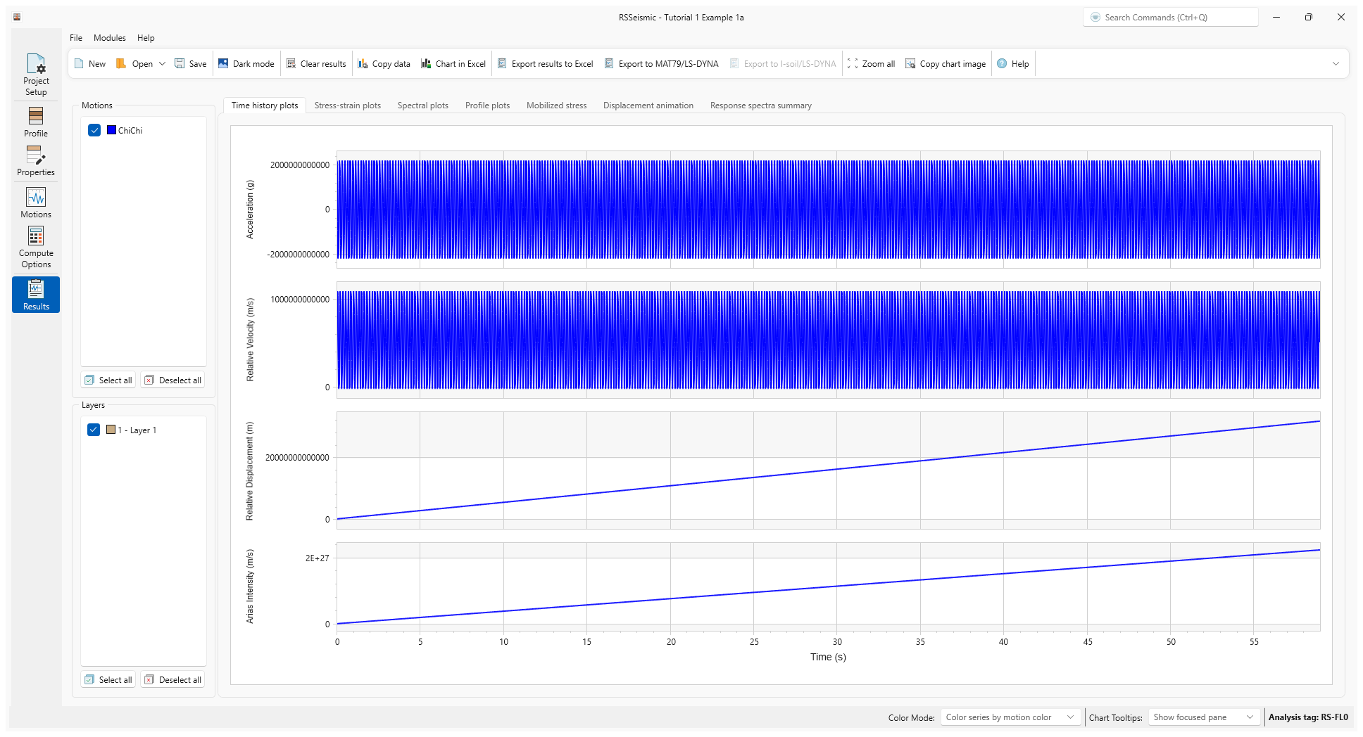
1. Select the Results tab

The Results section of RSSeismic contains a series of tabs that allow you to review the results of your analysis.

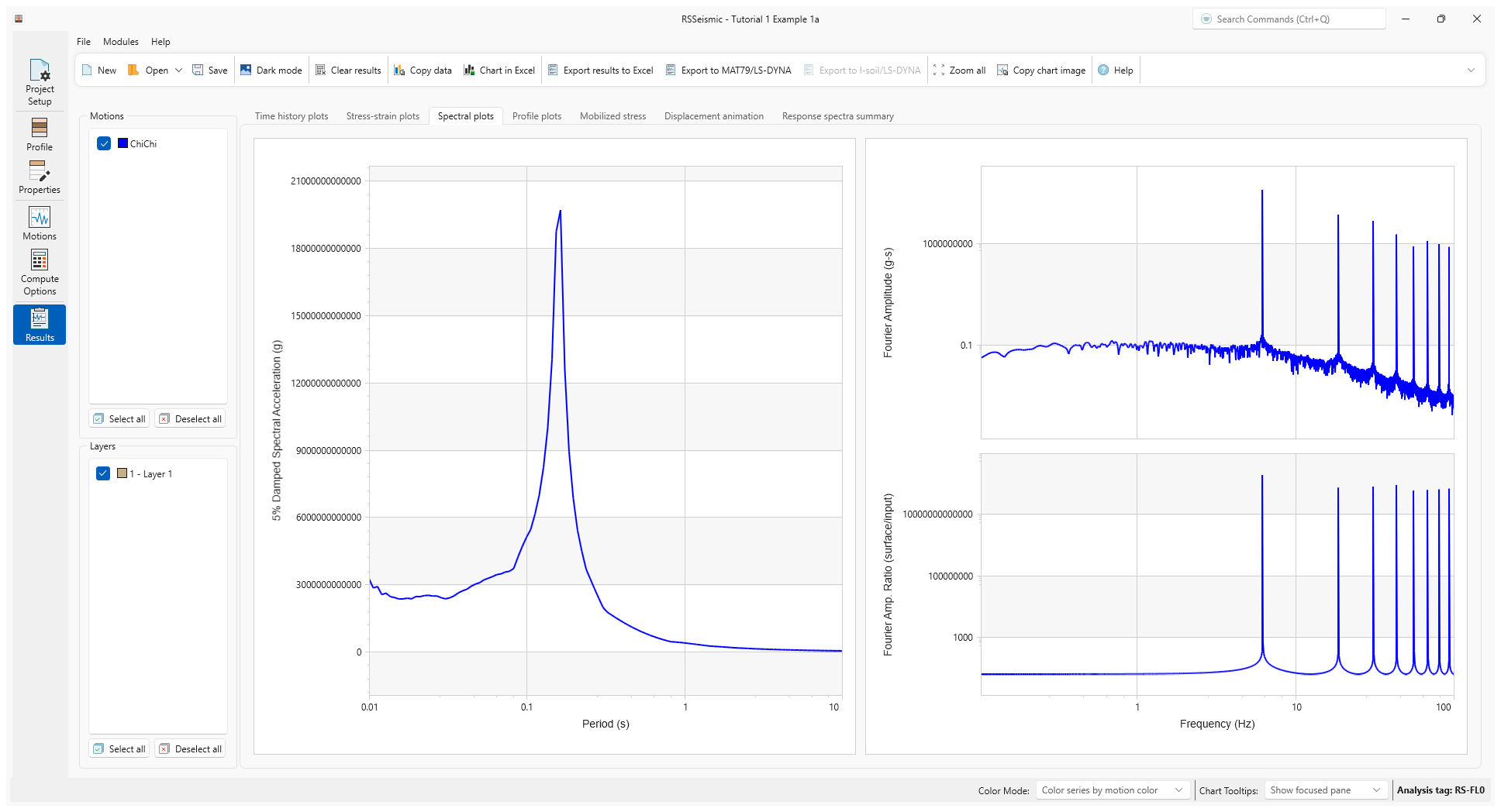
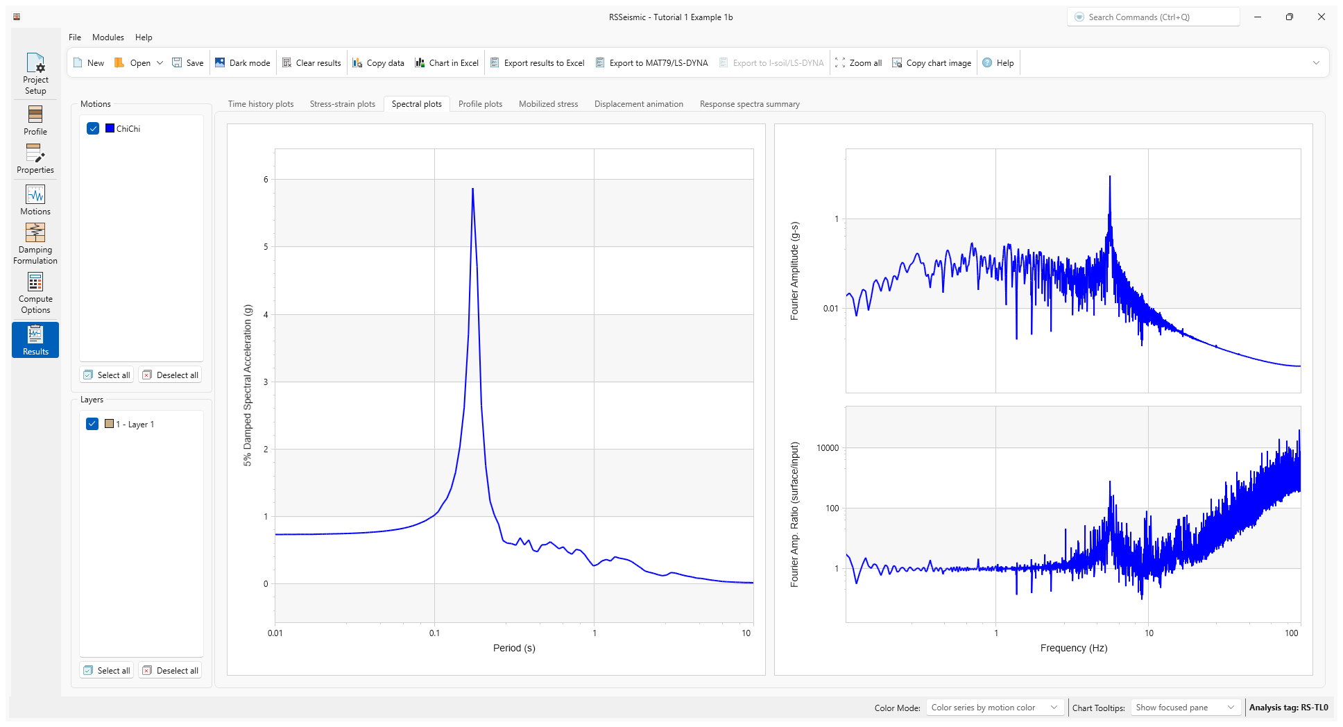
Below are the computed time-history (acceleration, velocity, displacement and arias intensity), and spectral plots (5% damped spectral acceleration, FAS and FAS ratio).

This being an undamped soil with rigid rock, the ground motions will be amplified to infinity (notice the very large accelerations) at a period equal to the period of the soil column. The natural period of the soil column is 0.16 sec (6.25 Hz). One can see that the response spectrum has a peak at 0.16 sec. The Fourier amplitude spectrum shows a first peak at the first mode of the soil column of 6.25 Hz. Additional peaks are seen at higher modes (multiples of 6.25Hz), such as the second mode at 12.5 Hz.

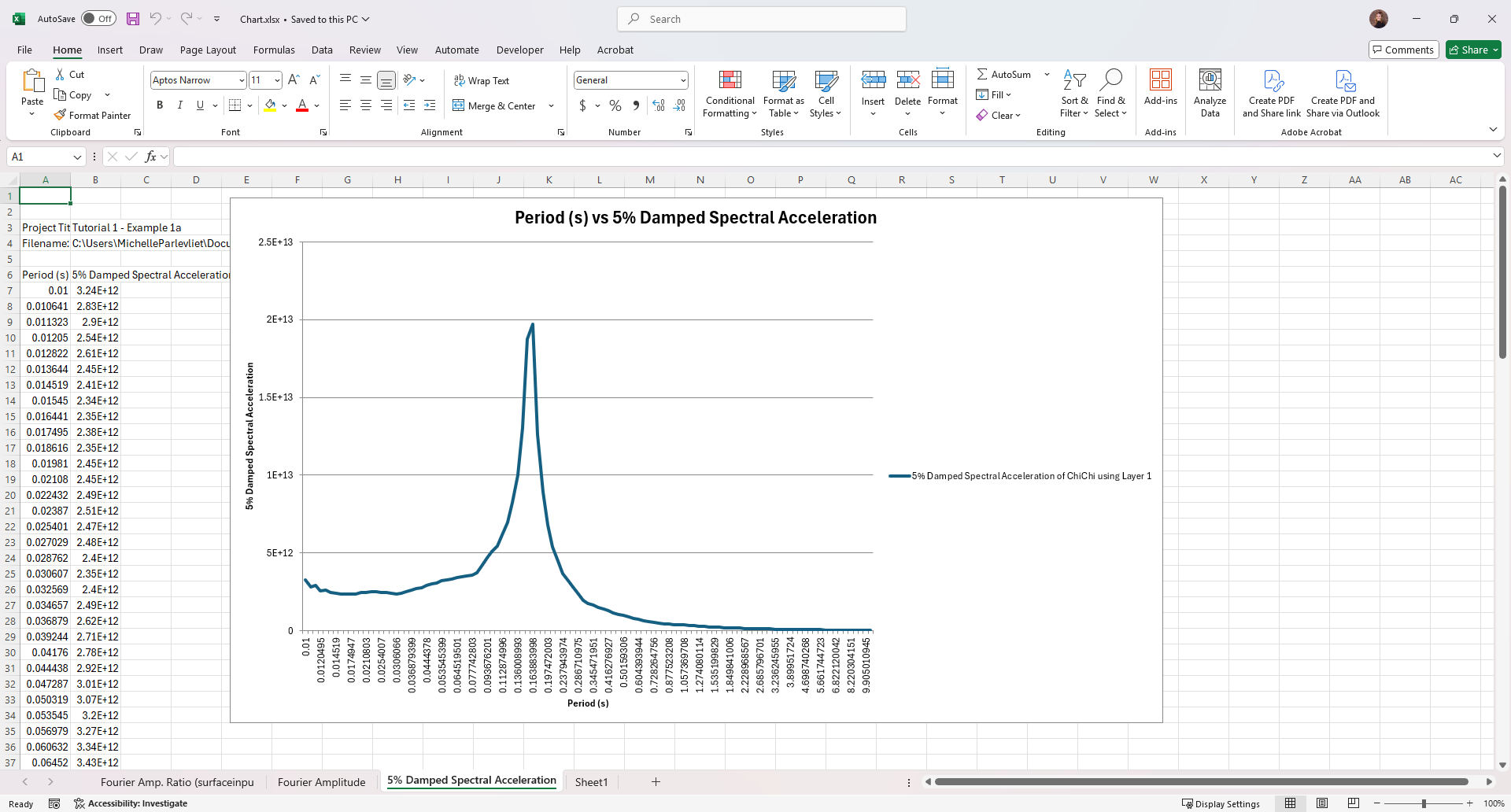
These results can be exported to Excel using the Chart in Excel option (located in the toolbar at the top of the window).

2. Click Chart in Excel
3. Enter a name for the Excel file and click Save.

Below is an example of the exported spectral plots.

3.0 Example 1b

Undamped Linear Analysis with Rigid Bedrock (Time Domain Solution)

Using the same soil profile and properties, we will now perform a Time Domain Linear Analysis.

3.1 Project Setup

1. Return to the Project Setup tab.
2. Select File > Save Project As and save this project as Tutorial 1 Example 1b.rsseismicfile.
3. Change the Solution Type to Time Domain.
4. The Damping Formulation tab will appear in lefthand navigation bar (beneath the Motions tab).

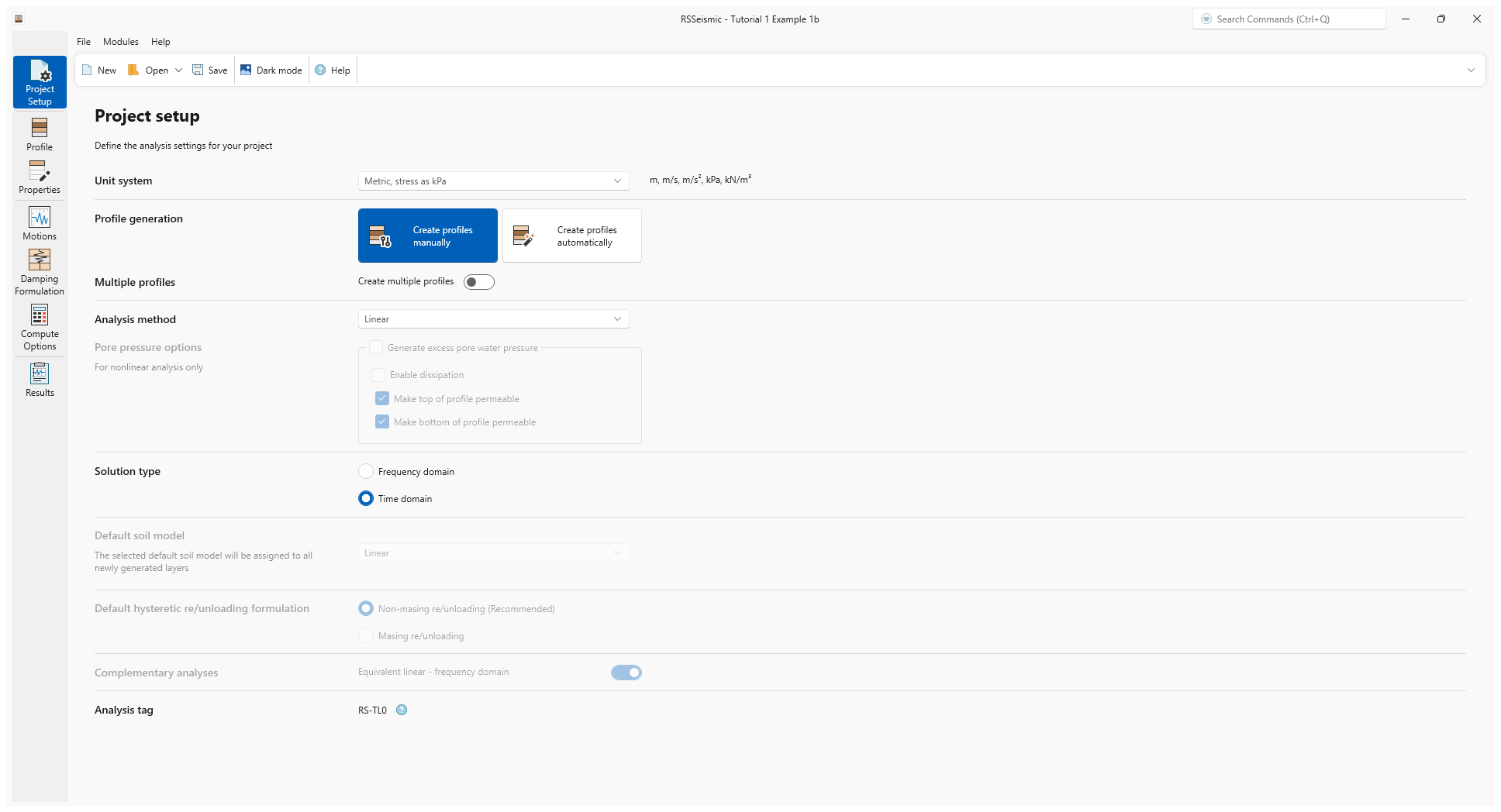
Notice at the bottom of the Project Setup that the Analysis Tag changes when you change your solution type. The Analysis tags are identifiers that are included in the analysis results to help users identify the kind of soil model analysis that RSSeismic performed. Click on the Info icon next to the Analysis tag ID to view the full table of analysis tags.

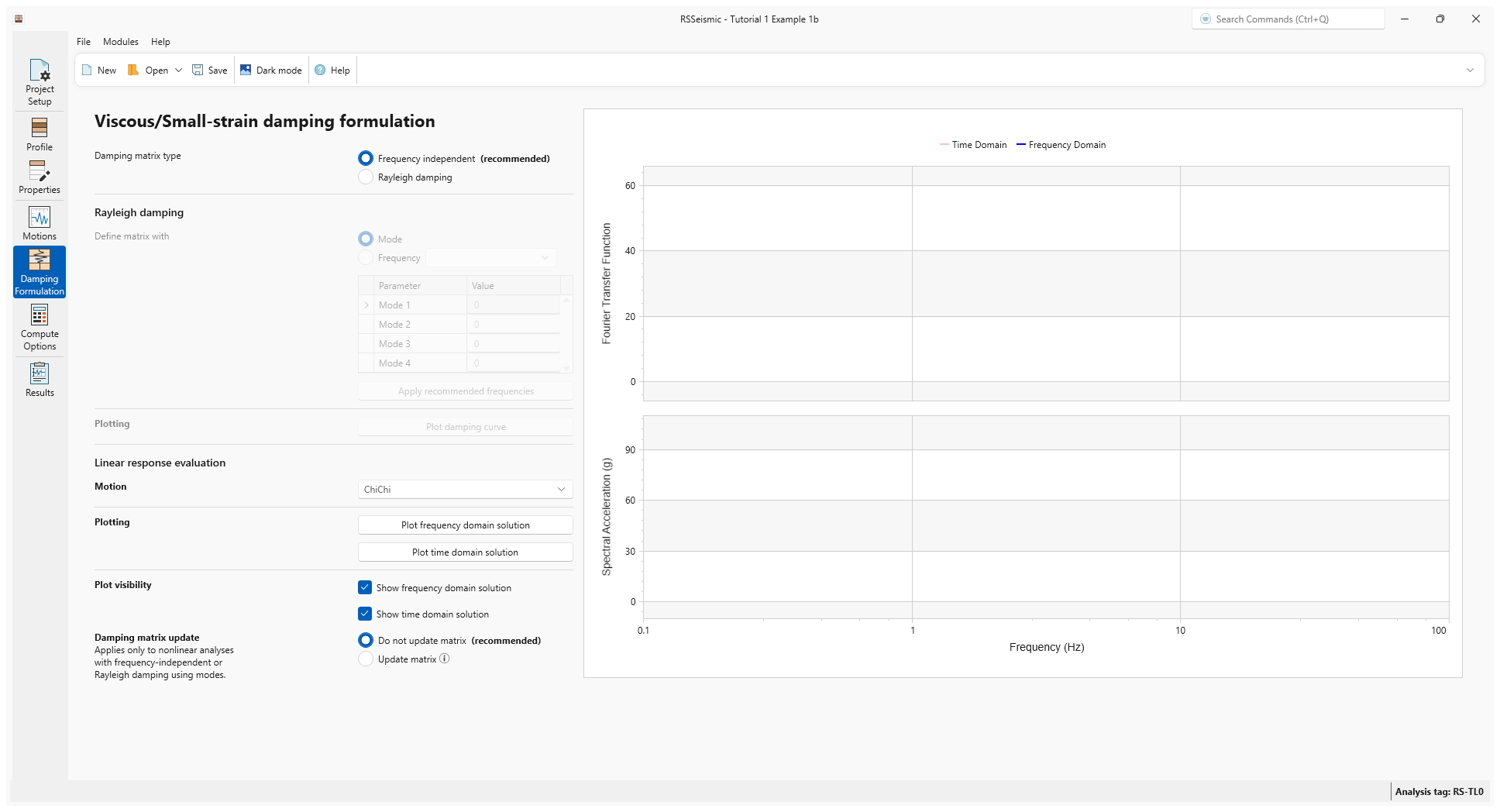
3.2 Damping Formulation

1. Select the Damping Formulation tab

The Viscous/Small-Strain Damping option is only available when a Time Domain analysis is being performed. We will use the default recommended Damping Matrix Type = Frequency independent option. For the Damping Matrix Update, the default Do not update damping matrix should remain selected.

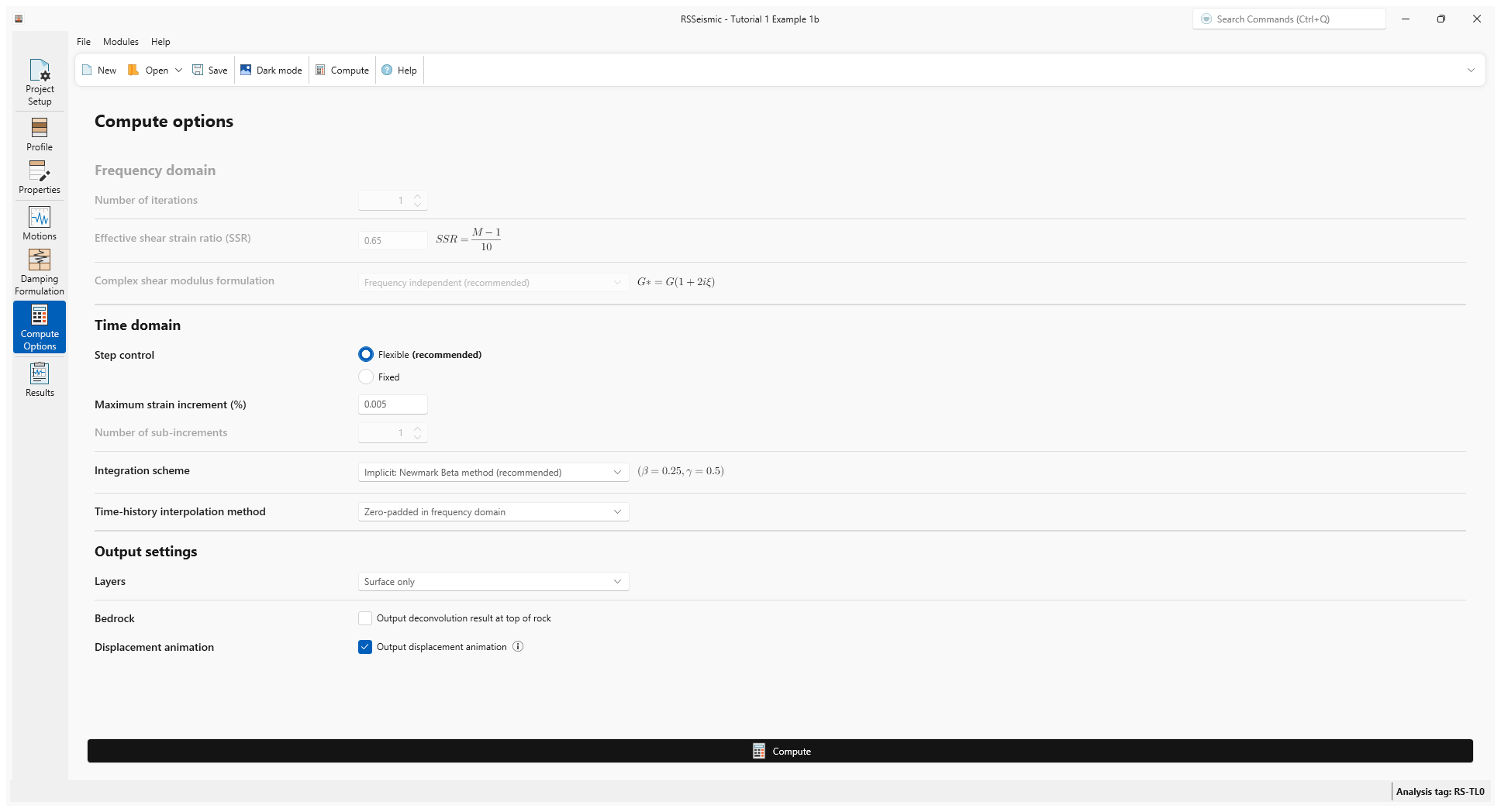
3.3 Compute

1. Select the Compute Options tab. Just like before, because we are now using a Time Domain solution, only the Time Domain options will be available.
2. For Time Domain enter:
   1. Step Control = Flexible
   2. Maximum strain increment (%) = 0.005
   3. Integration Scheme = Implicit: Newmark Beta Method (recommended)
   4. Time-History Interpolation Method = Zero-padded in frequency domain
3. Leave all other settings as is.
   
4. Click Compute.
5. Once the compute is completed, click Save in the toolbar at the top of the screen.

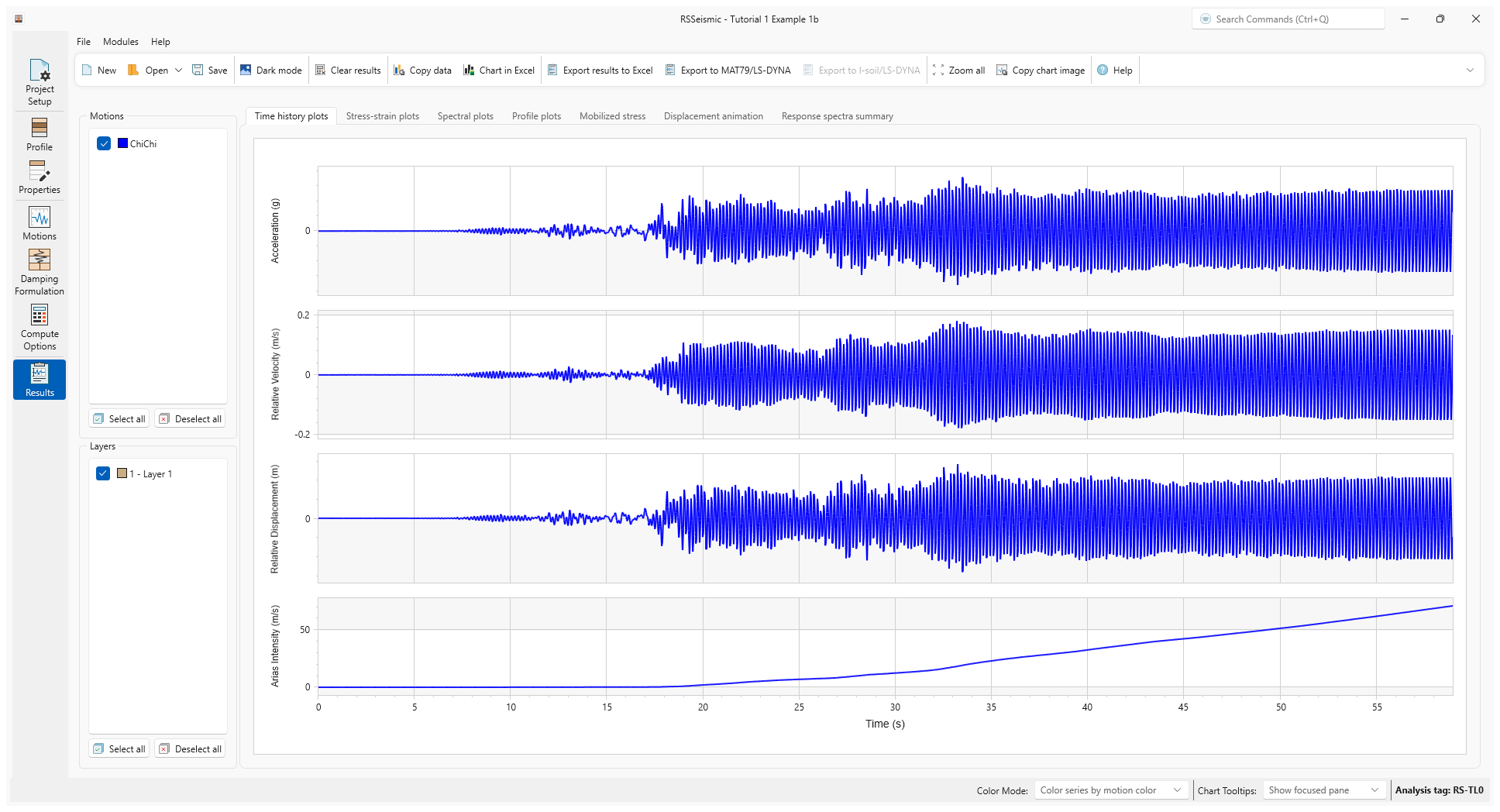
3.4 Results

1. Go to the Results tab
2. Click through the Time-histories and Spectral plots tabs to review the results.

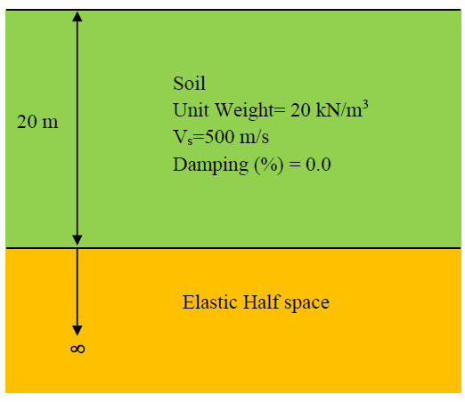
4.0 Example 2a

Undamped Linear Analysis with Elastic Bedrock (Frequency Domain Solution)

The second example is quite similar Example 1, except the bedrock definition has been changed to Elastic Half-space, and is defined as follows:

1. Shear wave velocity: 760 m/s
2. Unit weight: 25.0 kN/m3
3. Damping Ratio: 2.0 %

For most site response analysis problems, the ground motion is provided at an equivalent rock outcrop. In order to transfer the ground motion to the bottom of the column, still in the rock, using the elastic rock option will automatically accomplish this. For most site response analyses, users will use an elastic rock option.

From a numerical point of view, the use of an elastic rock, even with zero damping in soil, resonance as shown in Example 1 will not occur. This is also shown in broadly used textbook used in geotechnical earthquake engineering.

4.1 Project Setup

1. Return to the Project Setup tab
2. Select File > Save Project As and save this project as Tutorial 1 Example 2a.rsseismicfile.
3. Change the Solution type to Frequency Domain.

4.2 Properties

1. Go to the Properties tab
2. Select the Bedrock layer by either clicking on the soil profile on the left or using the drop down list.
3. Change the Halfspace option to Elastic Halfspace.
4. Enter the following:
   1. Shear wave velocity (m/s) = 760
   2. Unit weight (kN/m³) = 25.0
   3. Damping Ratio (%) = 2.0

4.3 Compute

1. Go to the Compute Options tab
2. Use the same compute options from section 2.5 Compute Options for Example 1a. Click Compute.
3. Once the project is computed, click Save

4.4 Results

1. Go to the Results tab
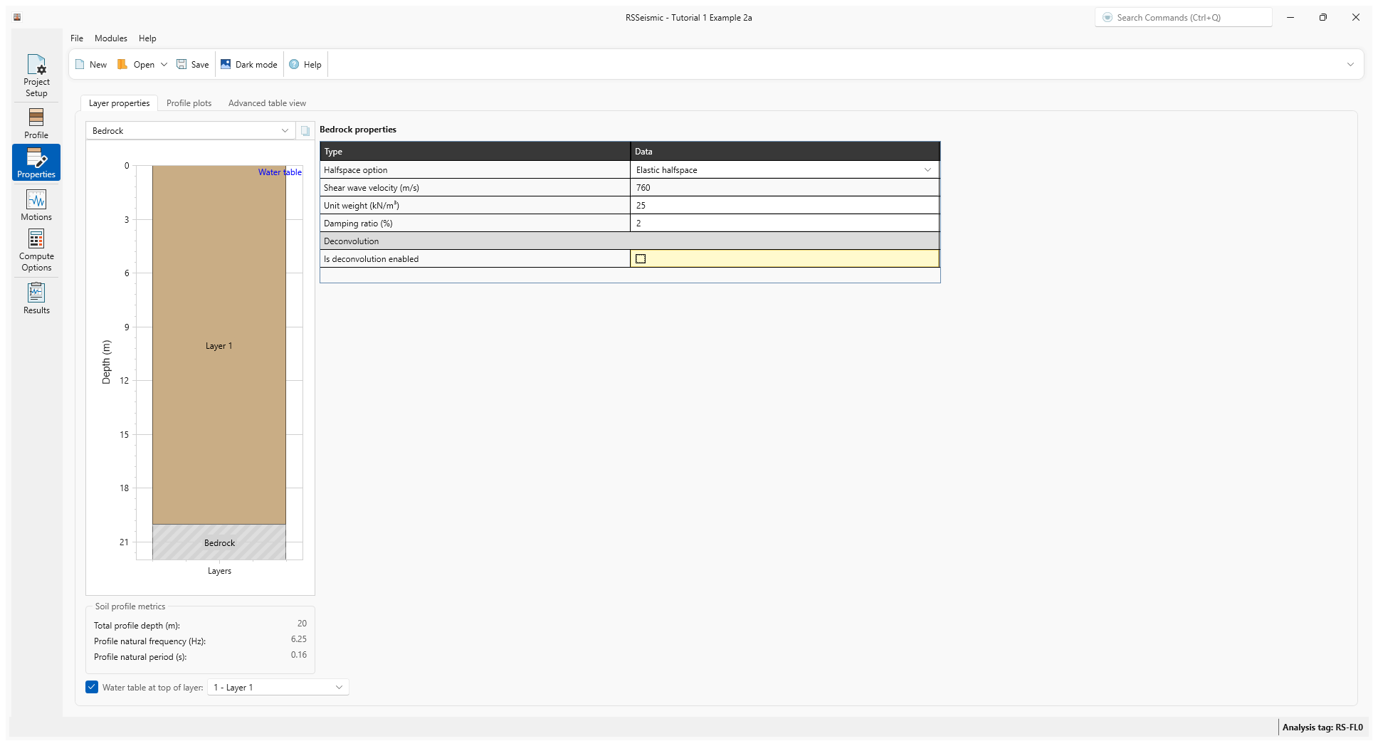
2. Below are the Time History Plots.
   The analysis results show much lower surface response compared to Example 1a. This illustrates the damping effect of using an elastic base/bedrock.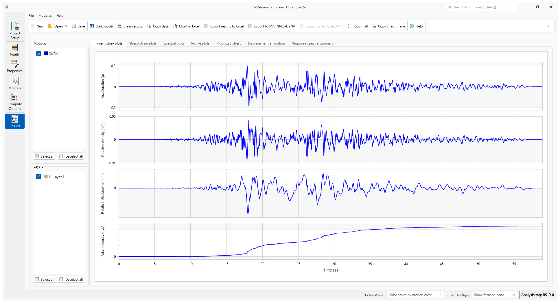
   
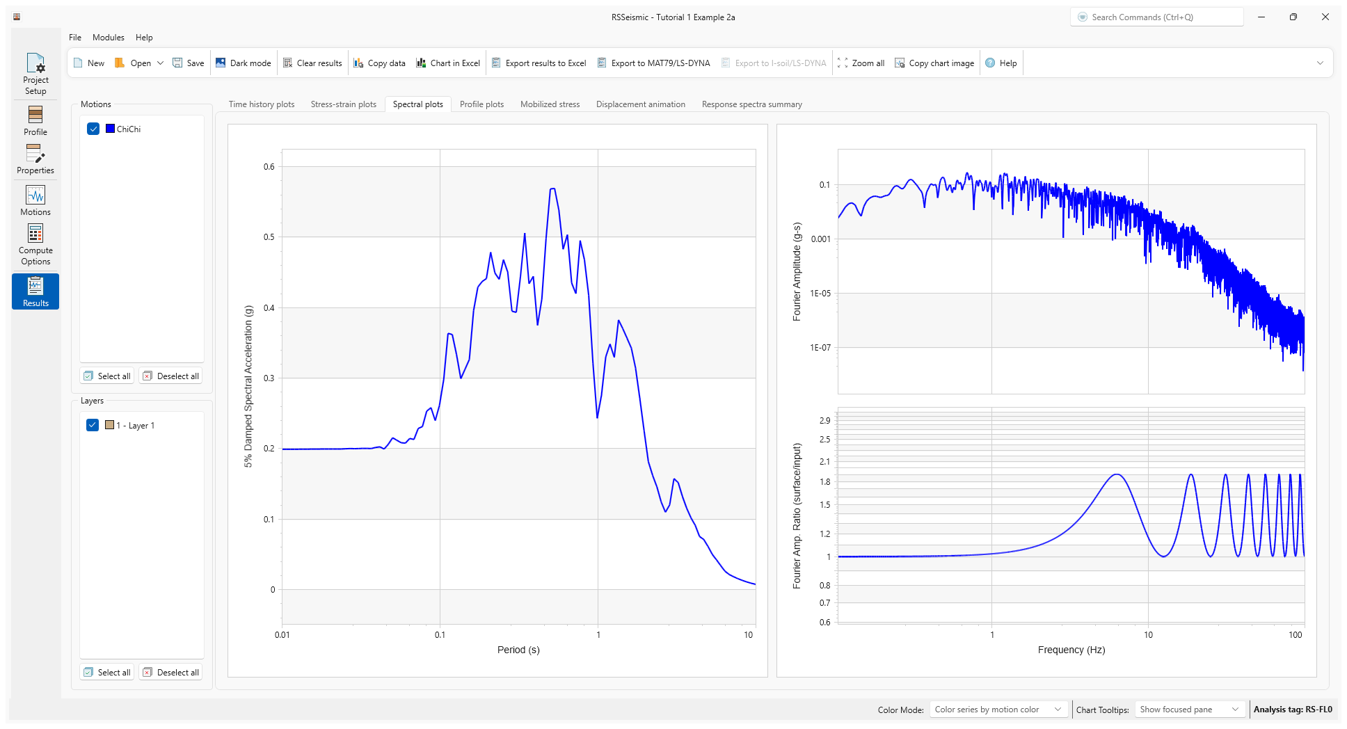
3. Select the Spectral Plots tab.
   

5.0 Example 2b

Undamped Linear Analysis with Elastic Bedrock (Time Domain Solution)

5.1 Project Setup

1. Go to the Project Setup tab
2. Select File > Save Project As and save this project as Tutorial 1 Example 2b.rsseismicfile.
3. Change the Solution type to Time Domain.

5.2 Damping Formulation

We will use the default recommended Damping Matrix Type = Frequency independent option. For the Damping Matrix Update, the default Do not update damping matrix should remain selected.

5.3 Compute

1. Go to the Compute Options tab
2. Leave all inputs as is and click Compute.
3. Once the project is computed, click Save

5.4 Results

1. Go to the Results tab.
2. Below are the Time History Plots.
   
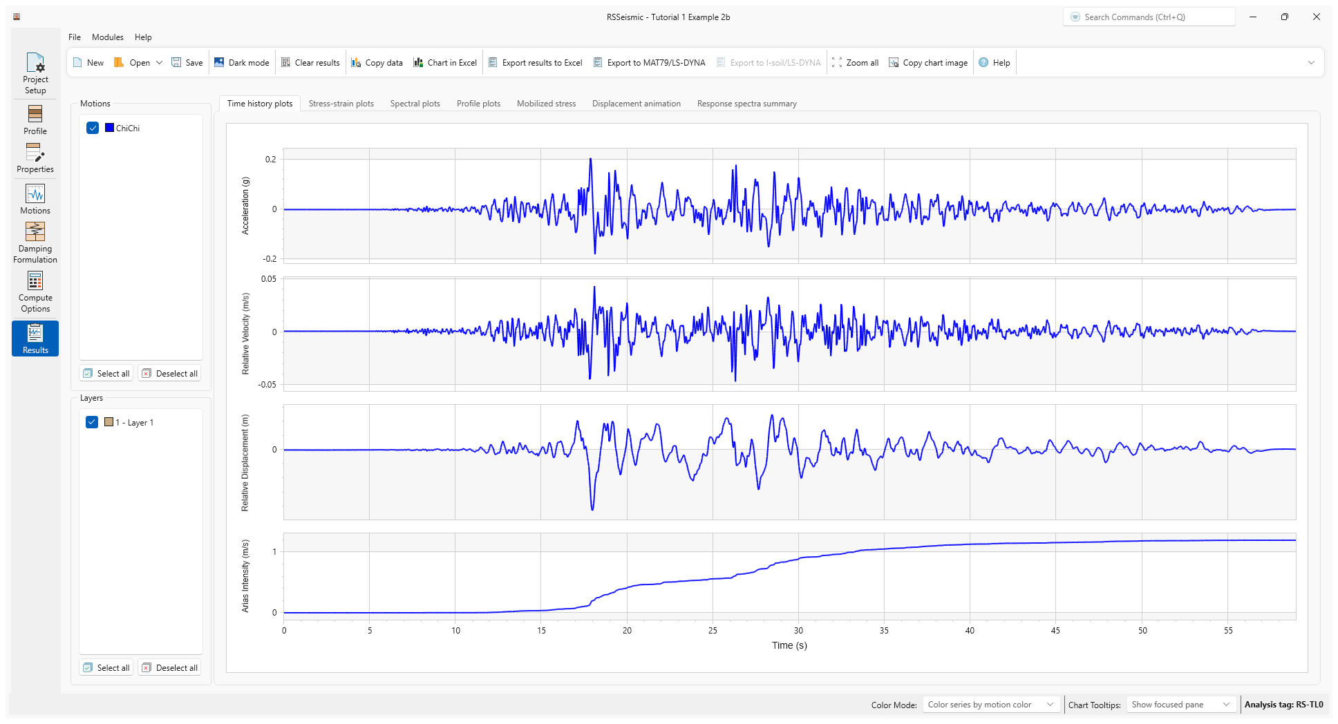
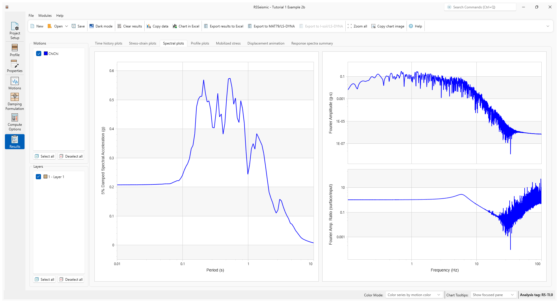
3. Select the Spectral Plots tab.

6.0 Example 3a

Damped Linear Analysis with Elastic Bedrock (Frequency Domain Solution)

In this example we build on the prior idealized examples, by adding a non-zero damping value to the example. This demonstrates the impact of damping on the computed surface response. We use 5% damping as a nominal value for a relatively stiff ground with linear response.

6.1 Project Setup

1. Return the Project Setup tab
2. Select File > Save Project As and save this project as Tutorial 1 Example 3a.rsseismicfile.
3. Change the Solution Type to Frequency Domain.

6.2 Properties

1. Go to the Properties tab
2. Ensure Layer 1 is selected.
3. Select the Soil Model Properties tab.
4. Enter Dmin (%) = 5.

6.3 Compute

1. Go to the Compute Options tab
2. Click Compute.
3. Once the project is computed, click Save

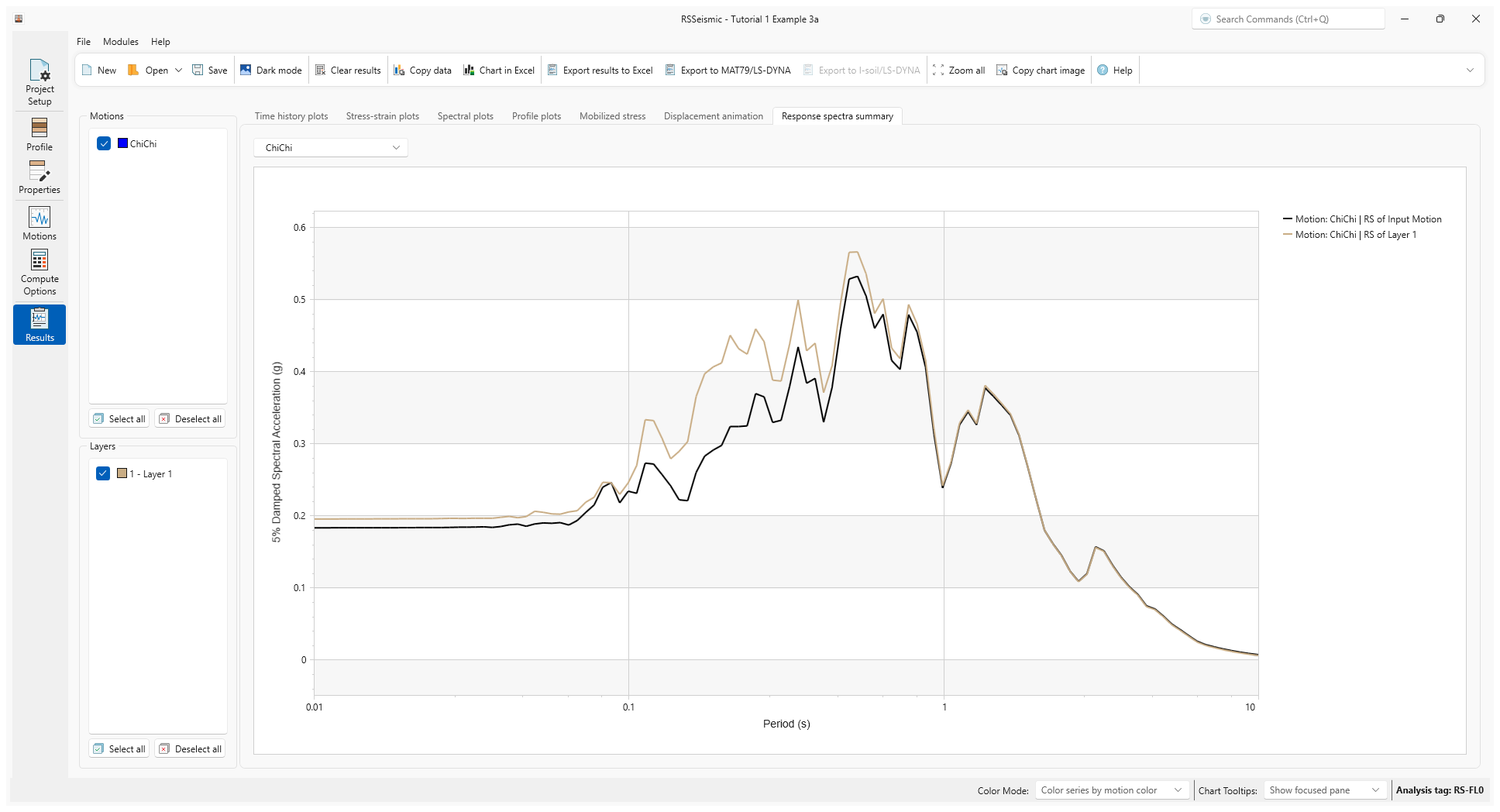
6.4 Results

1. Go to the Results tab
2. Below are the Time History Plots.
   
3. Select the Response Spectra Summary tab.
   

7.0 Example 3b

Damped Linear Analysis with Elastic Bedrock (Time Domain Solution)

7.1 Project Setup

1. Return to the Project Setup tab
2. Select File > Save Project As and save this project as Tutorial 1 Example 3b.rsseismicfile.
3. Change the Solution Type to Time Domain.

7.2 Damping formulation

We will use the default recommended Damping Matrix Type = Frequency independent option. For the Damping Matrix Update, the default Do not update damping matrix should remain selected.

7.3 Compute

1. Go to the Compute Options tab
2. Click Compute.
3. Once the project is computed, click Save

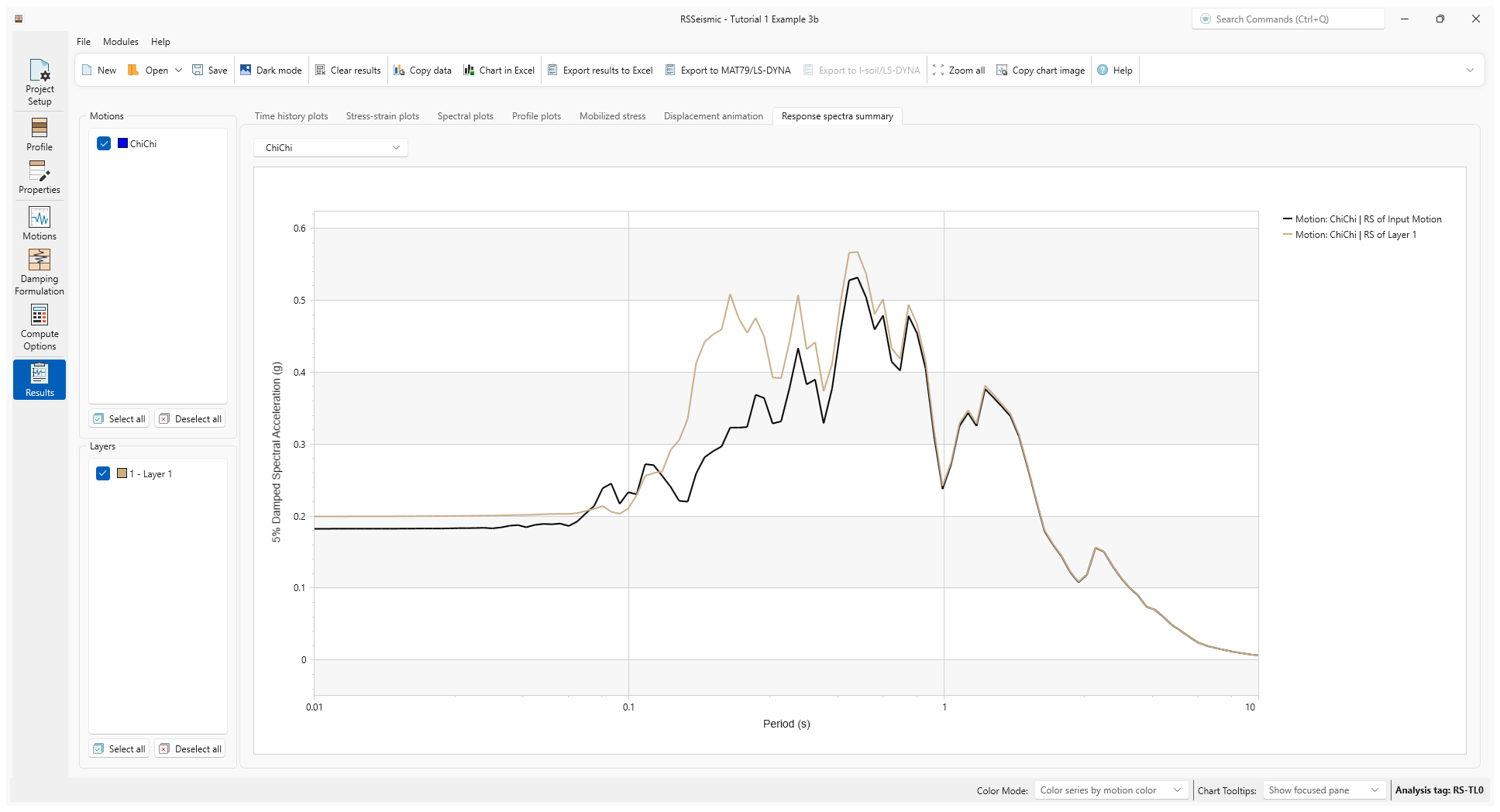
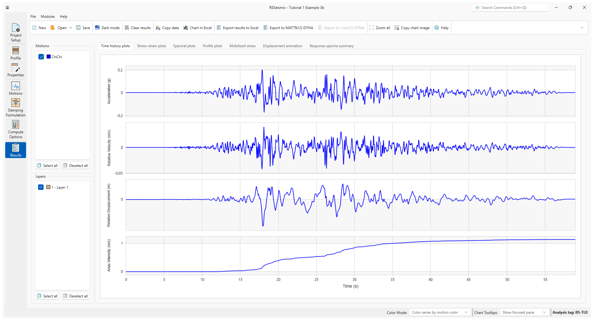
7.4 Results

1. Go to the Results tab
2. Below are the Time History Plots.
   
3. Select the Response Spectra Summary tab.