5 - Automatic Profile Generation

1.0 Introduction

This tutorial will demonstrate RSSeismic’s automatic profile generation feature, which allows users to (i) divide the soil layers considering the maximum frequency (f_max = V_S/4H), and (ii) automatically fit the selected soil model to reference dynamic soil curves for each layer.

When generating the soil profile, we will create a mean profile without randomization.

The site profile in this example is one of the 70,650 site profiles used in Harmon et al. (2017) and is composed of 20 clay layers with a constant unit weight of 19 kN/m³, PI = 15%, OCR = 1.5, and friction angle (𝜙) of 25⁰ along the profile. The shear wave velocity monotonically increases with depth and, shear strength required for fitting GQ/H Model at each layer is calculated the same as it was in Tutorial 3.

Topics covered in this tutorial:

• Automatic Profile Generation
• Mean Profile

Finished Product:

The finished product of this tutorial can be found in the Tutorial 5 folder. All tutorial files installed with RSSeismic can be accessed by selecting File > Recent Folders > Tutorials Folder from the RSSeismic main menu.

2.0 Project Setup

For this tutorial we will be performing a Nonlinear analysis on an automatically generated single soil profile with a GQ/H soil model. To begin:

1. Launch the RSSeismic program.
2. Select New Project . A new project will open, and you will be taken to the Project Setup tab.
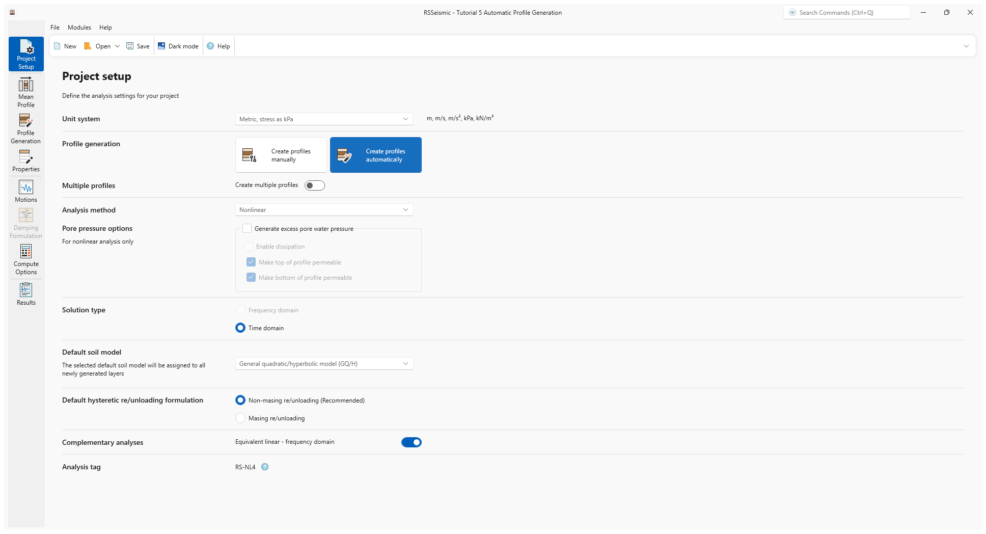
3. For Unit System select Metric, stress as kPa.
4. For Profile Generation select Create Profile Automatically.

Notice that the Profile tab has been replaced with two new tabs: Mean Profile and Profile Generation. We will be using these two tabs to generate the soil profile.

5. Since we are only creating one soil profile, leave Create multiple profiles turned OFF.
6. For the Analysis Method select Nonlinear.
7. For the Default Soil Model select General quadratic/hyperbolic model (GQ/H).
8. For Default hysteretic re/unloading formulation ensure the default Non-masing re/unloading (recommended) is selected.
9. For Complementary analyses, ensure Equivalent Linear – Frequency Domain is selected.

3.0 Mean Profile

1. Select the Mean Profile tab.

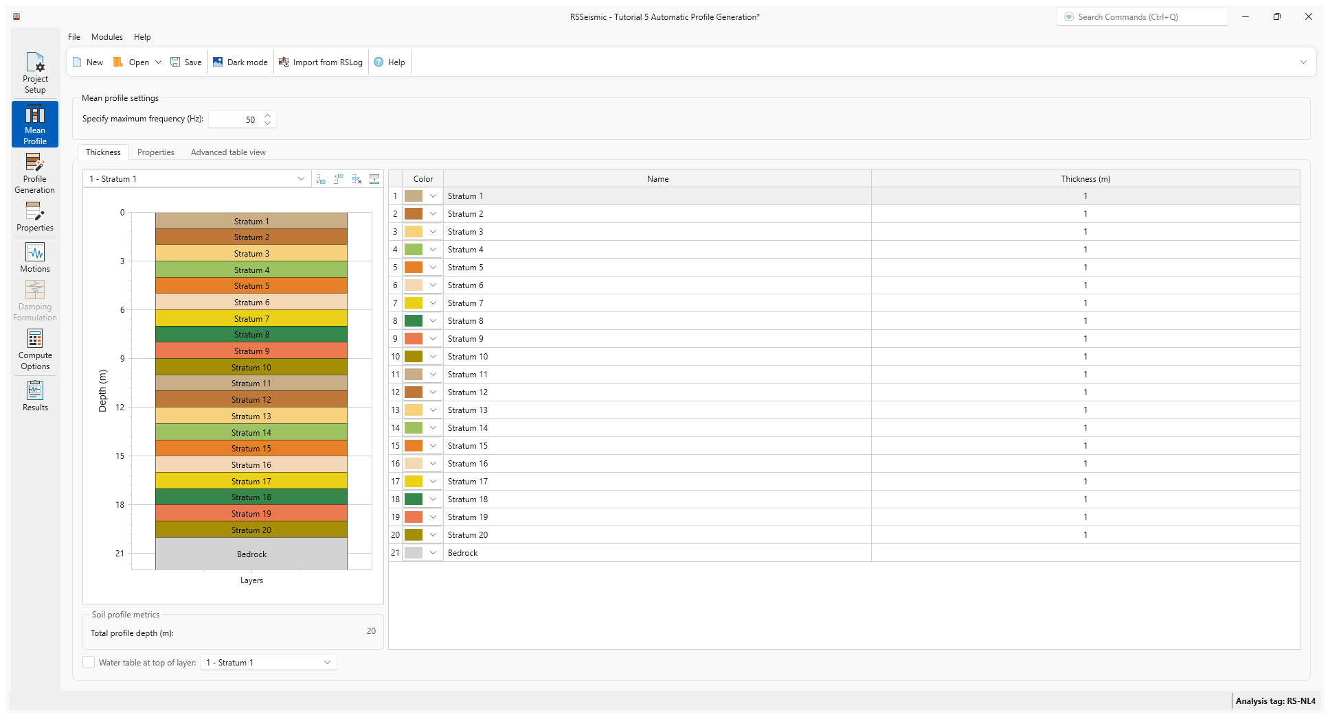
The Mean Profile tab is divided into 3 sections: Thickness, Properties, and Advanced Table View. We will use the Thickness and Properties sections to define the mean profile

2. At the top of the screen, the default Maximum Frequency (Hz) is provided as 50 Hz. This value is used to specify the maximum layer thickness. The selection of this maximum frequency depends also in part on the maximum frequency in the ground motion. In this example we chose the default value of 50 Hz.

Notice that for this Mean Profile, we are defining Stratum, rather than layers. We will define 20 strata. The intent of this step is to allow a user to define a geologically relevant strata. The automatic profile generation will then subdivide the stratum into layers.

3. Above the soil profile diagram click Append Rows, enter 19 and click OK. There should now be 20 rows.

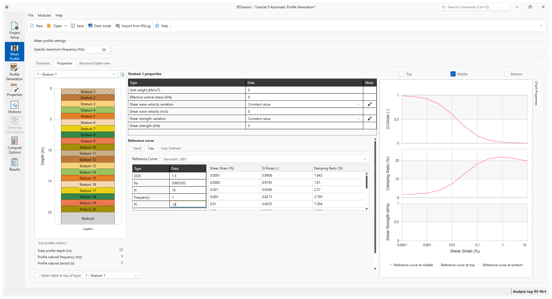
4. Select Properties. For Stratum 1, we will begin by entering the Reference Curve. Select the Clay tab.
5. Enter:
   1. Reference Curve = Darendeli, 2001
   2. OCR = 1.5
   3. Ko = 0.685302673
   4. N = 10
   5. Frequency = 1
   6. PI (Plasticity Index) = 15

6. In the top left of the screen next to the Stratum drop down list, there is a Copy properties option. Click Copy.
7. A dialog will appear, allowing you to copy the properties of Stratum 1 to the other 19 stratum. Ensure Stratum 2-20 are selected and click OK. Now the Reference curve data has been copied to all the stratums.
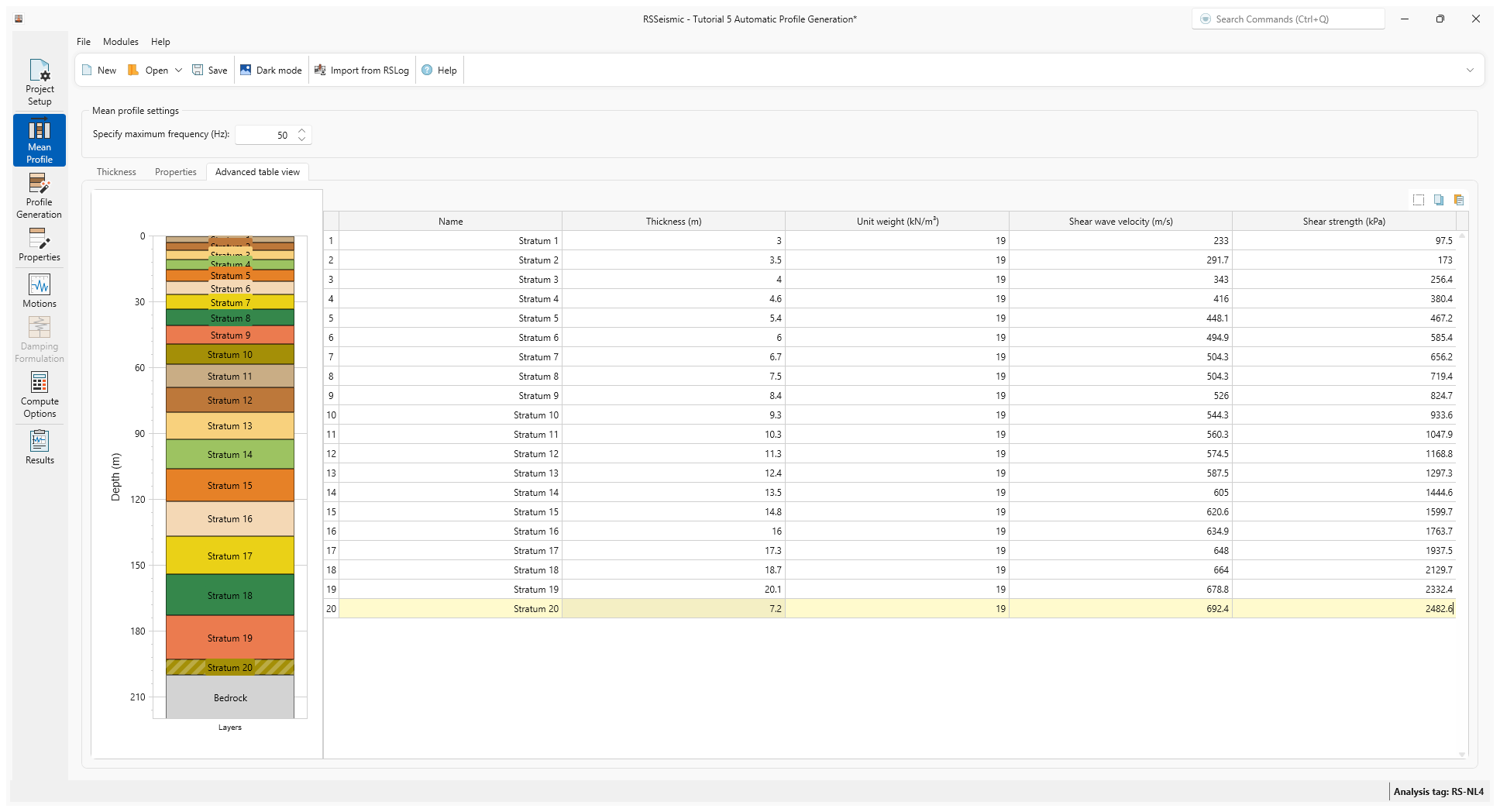
8. For the other stratum properties (including thickness, unit weight etc.), we will use the Advanced Table View to quickly add those parameters.
9. Copy and paste the values from the table below into the Advanced Table View. There is also a CSV of these values included in the Tutorial 5 folder.

Stratum Name	Thickness (m)	Unit Weight (KN/m^3)	Shear Wave Velocity (m/s)	Shear Strength (kPa)
Stratum 1	3	19	233.	97.5
Stratum 2	3.5	19	291.7	173.
Stratum 3	4.	19	343.0	256.4
Stratum 4	4.6	19	416	380.4
Stratum 5	5.4	19	448.1	467.2
Stratum 6	6	19	494.9	585.4
Stratum 7	6.7	19	504.3	656.2
Stratum 8	7.5	19	504.3	719.4
Stratum 9	8.4	19	526	824.7
Stratum 10	9.3	19	544.3	933.6
Stratum 11	10.3	19	560.3	1047.9
Stratum 12	11.3	19	574.5	1168.8
Stratum 13	12.4	19	587.5	1297.3
Stratum 14	13.5	19	605	1444.6
Stratum 15	14.8	19	620.6	1599.7
Stratum 16	16	19	634.9	1763.7
Stratum 17	17.3	19	648	1937.5
Stratum 18	18.7	19	664	2129.7
Stratum 19	20.1	19	678.8	2332.4
Stratum 20	7.2	19	692.4	2482.6

10. Go to the Properties section and select Stratum 1. The properties will now be as follows:
    1. Unit weight (kN/m³) = 19
    2. Shear wave velocity variation = Constant value
    3. Shear wave velocity (m/s) = 233
    4. Shear strength variation = Constant value
    5. Shear strength (kPa) = 97.5
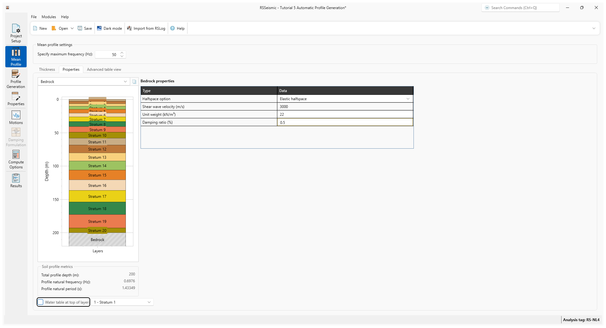
11. Select the Bedrock layer.
12. Under Bedrock properties enter:
    1. Halfspace option = Elastic Halfspace
    2. Shear wave velocity (m/s) = 3000
    3. Unit weight (kN/m³) = 22
    4. Damping Ratio (%) = 0.5

4.0 Profile Generation

1. Go to the Profile Generation tab

As mentioned before, for this initial profile we will not be using Randomization.

2. Click Generate Profiles.

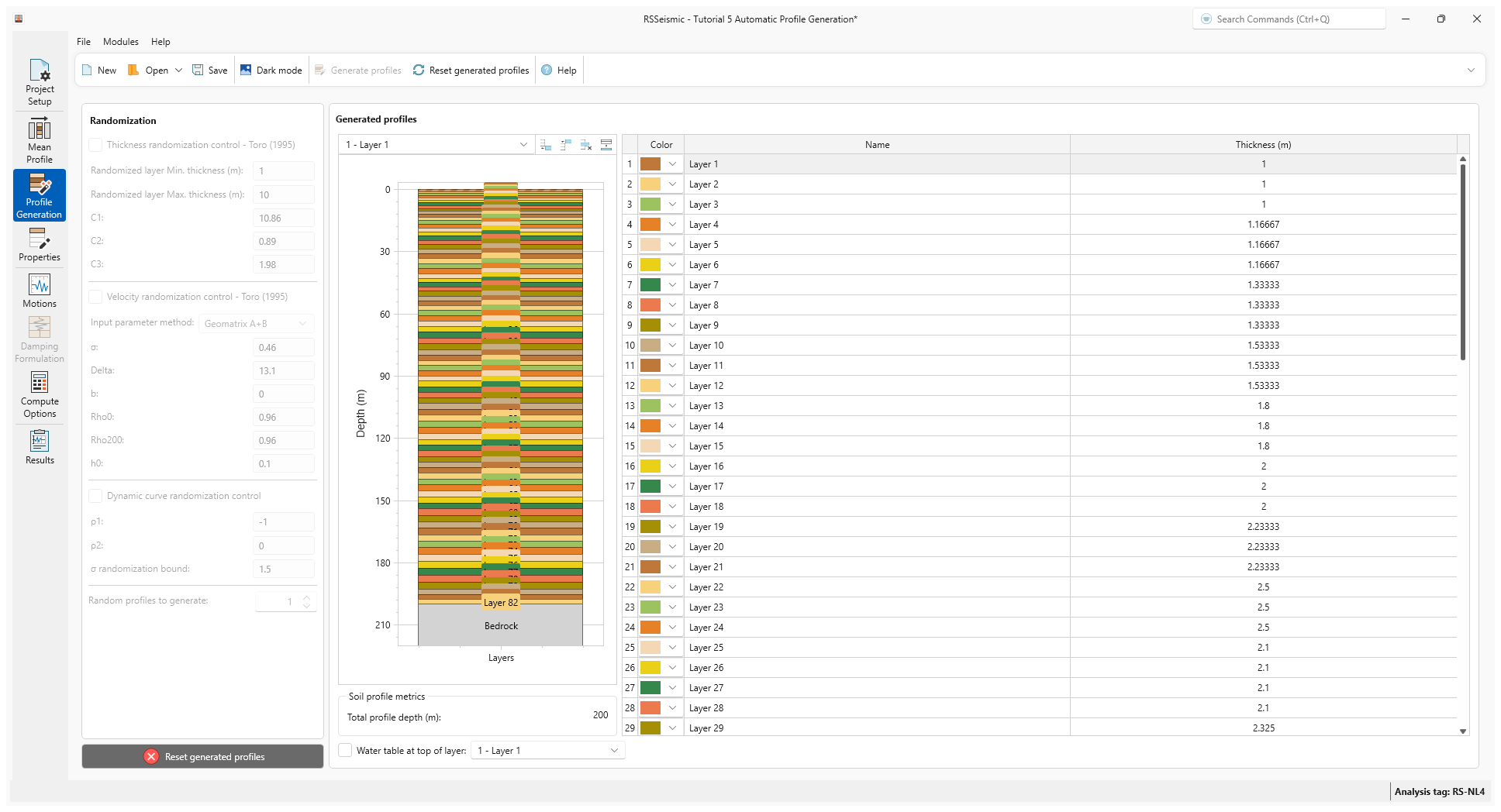
A profile consisting of 82 layers will be generated. You will notice that the top layers are less than 1 m thick as the shear wave velocity is small, and hence a thinner layer is needed to achieve the target maximum frequency through the soil.

5.0 Properties

1. Go to the Properties tab
   
2. The Layer 1 properties with the reference curve data are shown below:

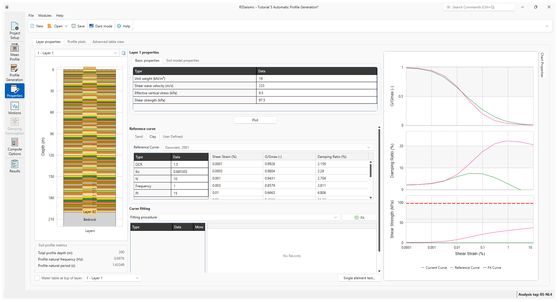
This fitting is performed automatically as part of the profile generation

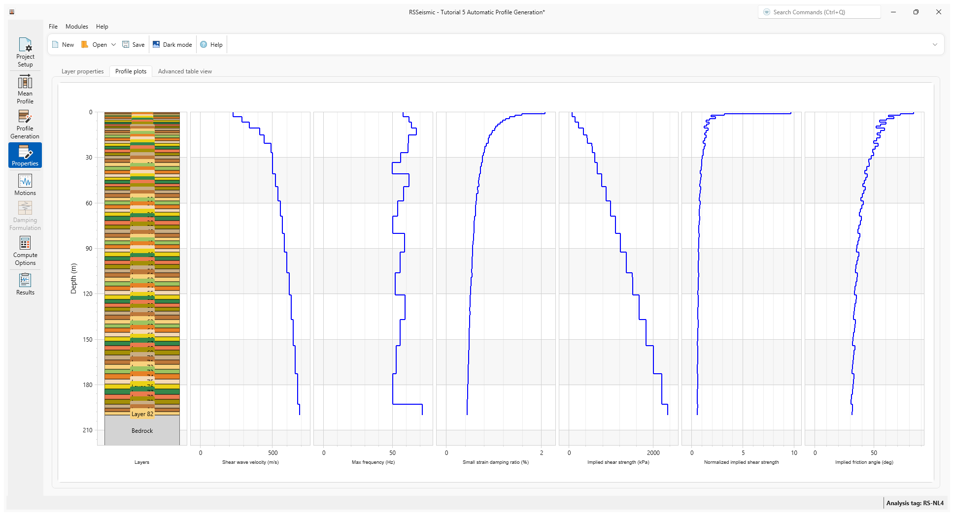
3. Select the Profile Plots tab to review the soil profile plots.

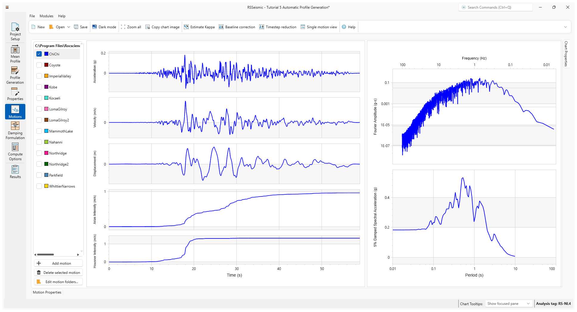
6.0 Motions

1. Select the Motions tab
   
2. Under Resources\Input Motions select ChiChi.

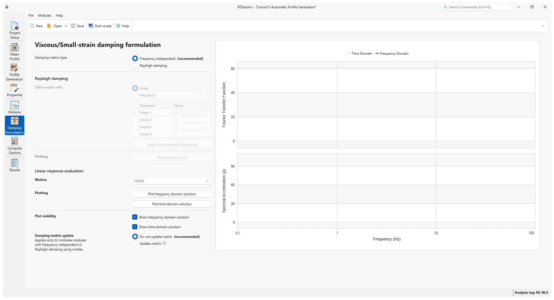
7.0 Damping Formulation

1. Select the Damping Formulation tab
   
2. We will use the default Frequency-independent viscous-damping along with No update in damping matrix selected.
3. At this point we will want to save the project. Select File > Save and save the project as Tutorial 5 Automatic Profile Generation

8.0 Compute options

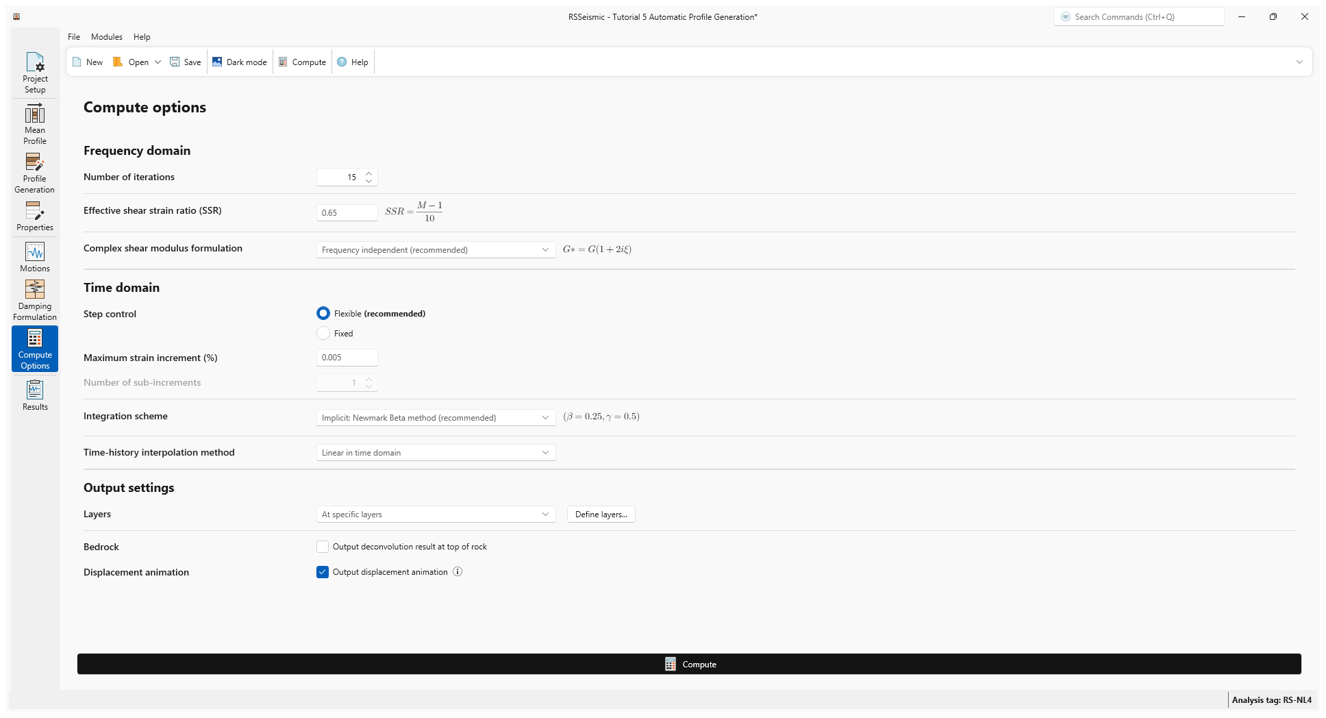
1. Go to the Compute Options tab
   
2. For the parameters for the nonlinear and equivalent-linear analyses, we use the defaults, which are as follows:
   • For frequency-domain analysis:
     • Number of iterations = 15
     • Effective Shear Strain Ratio (SSR) = 0.65
     • Complex Shear Modulus Formulation = Frequency-Independent
   • For nonlinear time-domain analysis:
     • Step Control = Flexible
     • Maximum Strain Increment (%) = 0.005
     • Integration Scheme = Implicit Newmark Beta Method
     • Time History Interpolation Method = Linear in time domain
3. For Output Settings select At specific layers.
4. Click Define Layers.
5. Click Deselect All and then select Layer 1. Click OK.
6. Click Compute.
7. Once the compute is completed, click Save .

9.0 Results

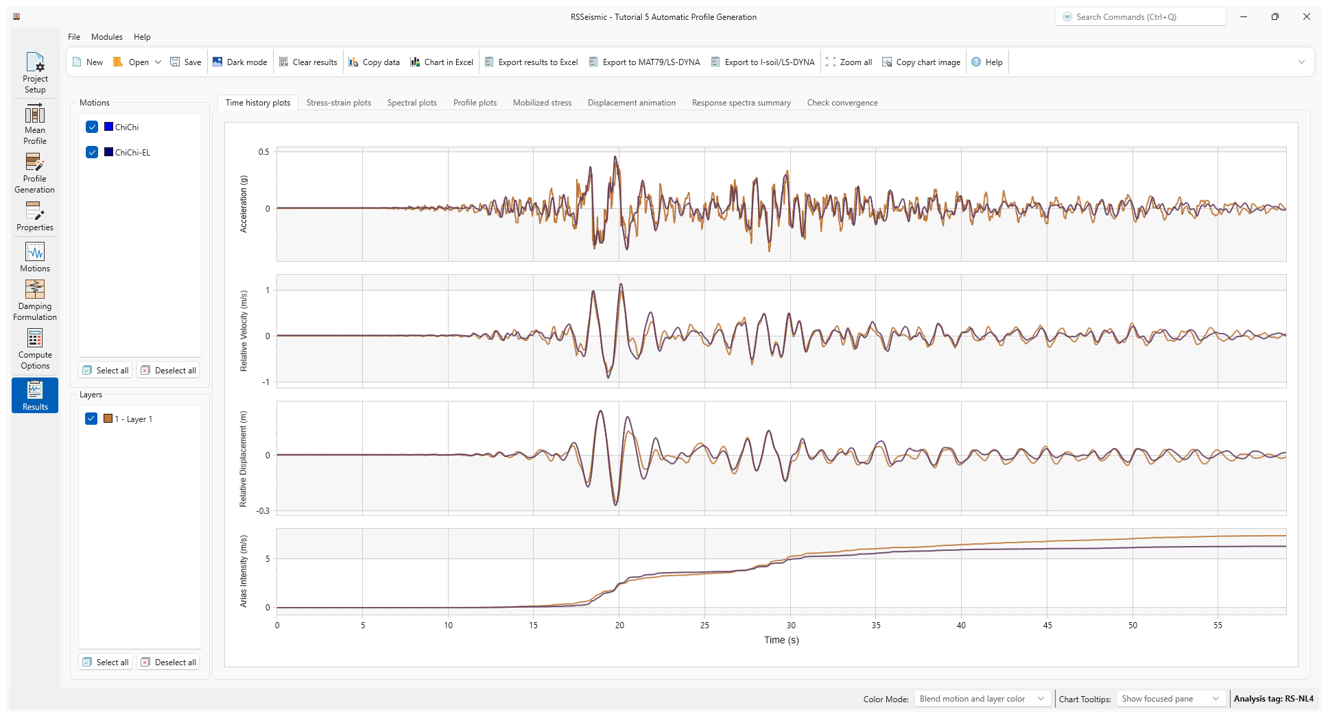
1. Go to the Results tab
   

Computed time-histories (acceleration, velocity, displacement and Arias Intensity) from nonlinear and equivalent-linear analyses are shown below.

2. Change the Color Mode to Blend motion and layer color to more easily see the lines.

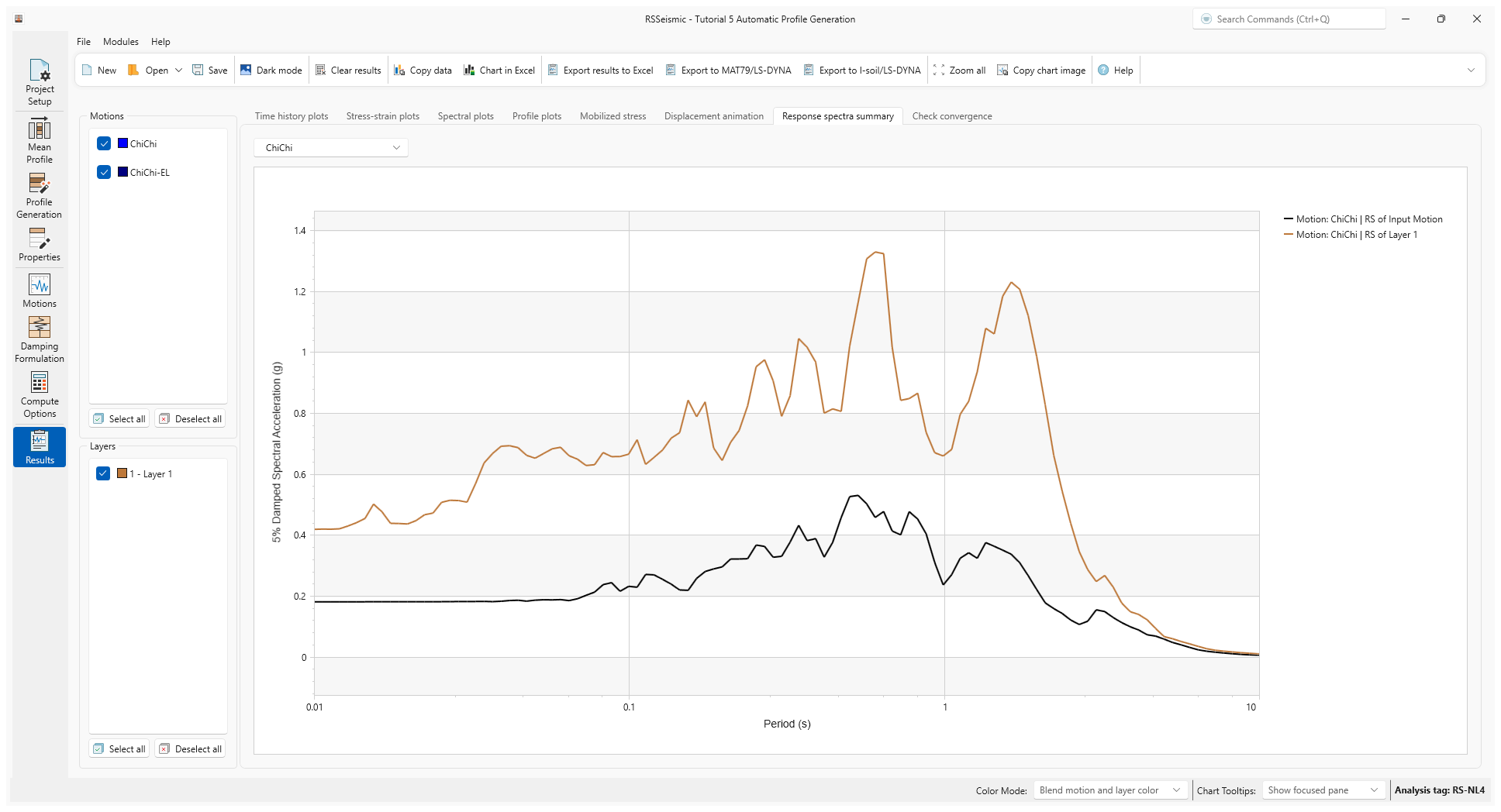
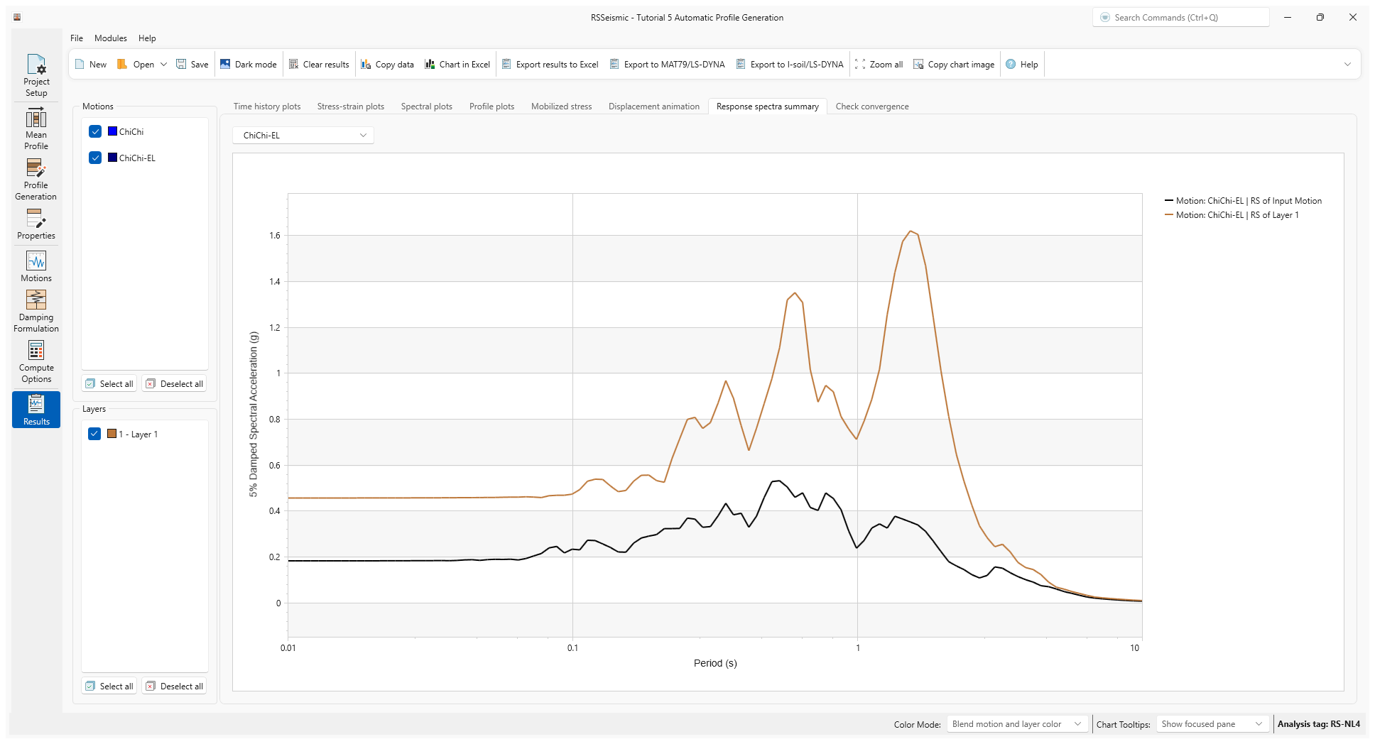
3. Select the Response Spectra Summary tab.
4. Use the drop down to switch between the Nonlinear and Equivalent Linear. 5% damped spectral acceleration at the top of the layer along with that of input motion from nonlinear and equivalent-linear analysis are show below.