2 - Equivalent Linear Analysis with Discrete Points

1.0 Introduction

For this tutorial, we will be performing an Equivalent Linear analysis with Frequency Domain. This procedure was developed in the late 1960s and early 1970s. It became widely adopted in engineering applications via the program SHAKE (Schnabel et al, 1972) and SHAKE 91 (Idriss and Sun, 1992). SHAKE used discrete points to define the soil dynamic curves (Normalized shear modulus and damping curves versus shear strain). Through this tutorial we demonstrate how the user can perform a "SHAKE" like analysis within a modern, and computationally efficient user interface and computational platform, RSSeismic.

In the first example we demonstrate the capability for a single soil layer soil column. In Section 8, we provide an additional exercise with multiple layers.

Topics covered in this tutorial:

• Equivalent Linear Frequency Domain analysis
• Discrete Points

Finished Product:

The finished product of this tutorial can be found in the Tutorial 2 folder. All tutorial files installed with RSSeismic can be accessed by selecting File > Recent Folders > Tutorials Folder from the RSSeismic main menu.

2.0 Project Setup

1. Begin by opening the RSSeismic program and selecting New Project
   

A new project will open and you will be taken to the Project Setup tab.

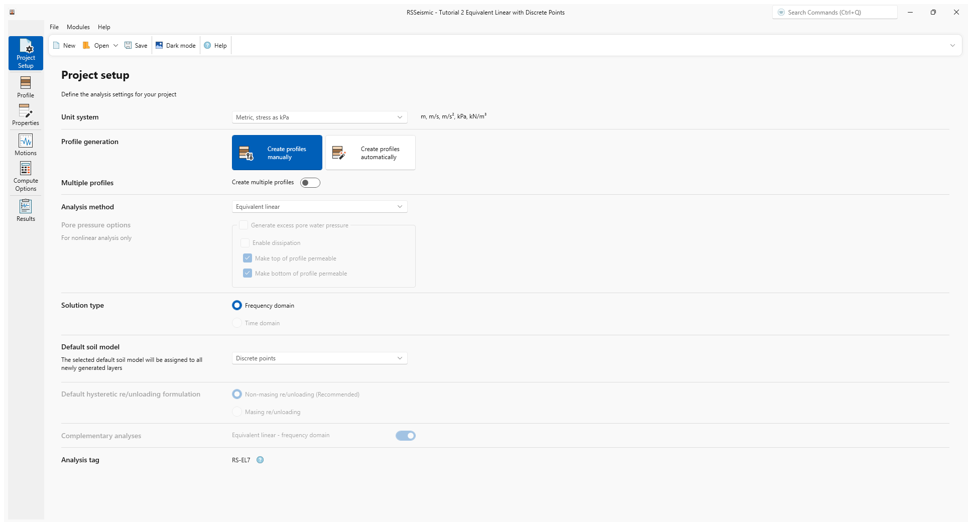
The Project Setup tab is used to configure the main setup parameters for your RSSeismic project. The Project Setup should always be selected before you proceed with creating your project, as some of the settings (for example, the Units System and Analysis Method) determine the inputs and availability of other options.

For this tutorial we will first be selecting an Equivalent Linear Frequency Domain analysis.

2. Before proceeding with the project parameters, save your project. Select File > Save Project and save your project as Tutorial 2 Equivalent Linear with Discrete Points.
3. Set the Unit System to Metric, stress as kPa.
4. For the Profile Generation, we will be leaving the default: Create Profiles Manually. Since we are only defining one soil profile, Create Multiple Profiles will remain turned off.
5. For the Analysis Method select Equivalent Linear.
6. For the Solution Type, only the Frequency Domain option is available when doing an Equivalent Linear analysis.
7. For the Default Soil Model select Discrete Points.

3.0 Profile

1. Go to the Profile tab
   

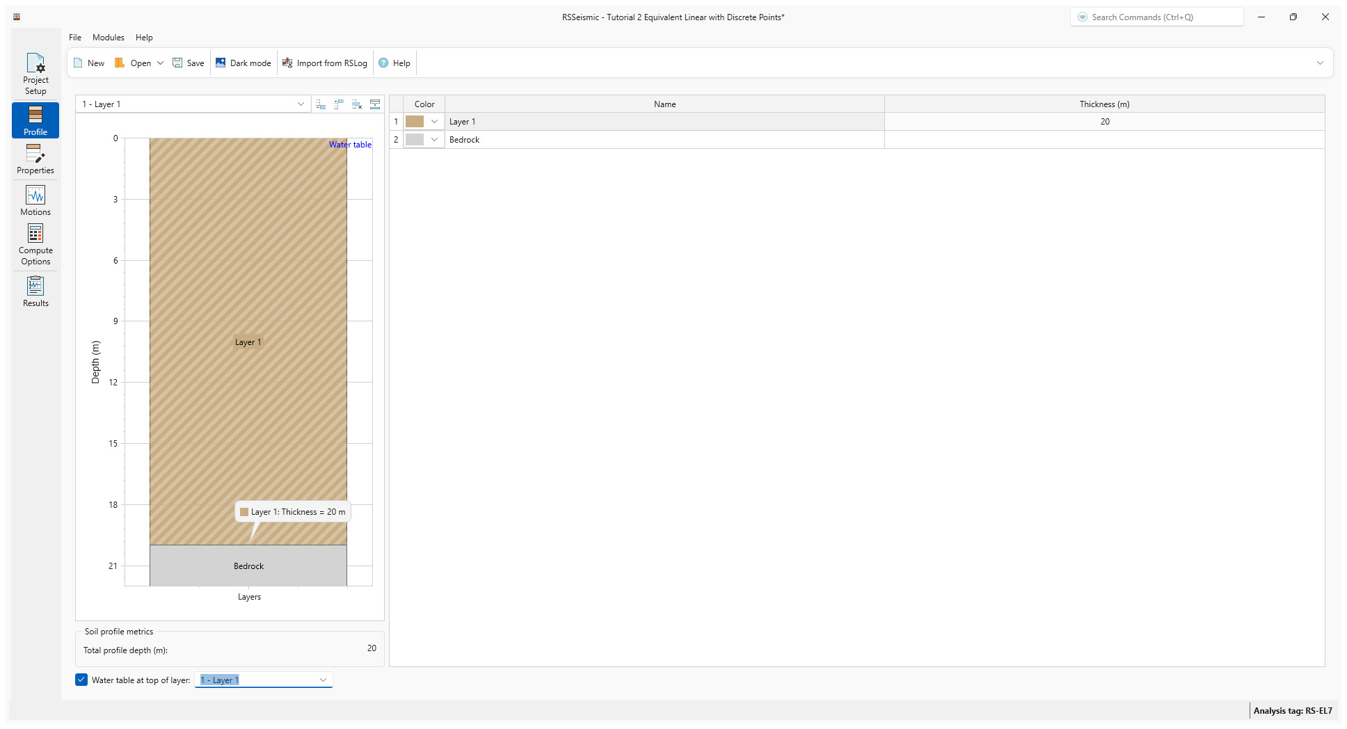
The Profile tab is used to define the basic stratigraphy of your soil profile. Users can add/remove layers and define the thickness of each layer. Further soil property details are defined in the Properties tab (which we will address in the next section).

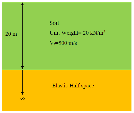
2. In the table on the right, select Layer 1 and enter a Thickness of 20 m.
3. In the bottom left of the screen, select Water table at top of layer and ensure Layer 1 is selected.

The Soil profile diagram on the left should update automatically, as should the Soil Profile Metrics below.

4.0 Properties

1. Go to the Properties tab
   

The Properties tab is used for defining the soil models for your soil profile. Users input their soil properties (unit weight, shear wave velocity, effective vertical stress) for each selected soil layer. Layer 1 should be selected by default. To switch layers, use the drop down list in the top left of the Layer Properties tab.

2. Ensure the Layer Properties tab is selected.
3. For Layer 1, under Basic Properties enter:
   1. Unit Weight (kN/m³) = 20
   2. Shear Wave Velocity (m/s) = 500
4. Select the Soil model properties tab. Notice that Discrete Points has been automatically selected as the soil model.
   In this tutorial we will use the Seed and Idriss, 1970 curves for sand to define the dynamic behavior of the soil. The normalized shear modulus versus shear strain curve reflects the reduction in shear modulus with increasing shear strain, while the damping curve versus shear strain reflects the increase in soil damping with increasing strain. The curves are commonly discretized as individual points and entered into a table as shown here. The resulting graph shows the curves plotted by connecting these pointsoints.
5. Enter:
   1. Dmin (%) = 0.48
   2. Click the Edit icon next to Discrete Points. The Define Discrete Points dialog will appear.
   3. Click the Append Rows button and add 11 rows for the Discrete Points.
   4. Enter the following and then click OK.

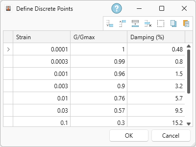
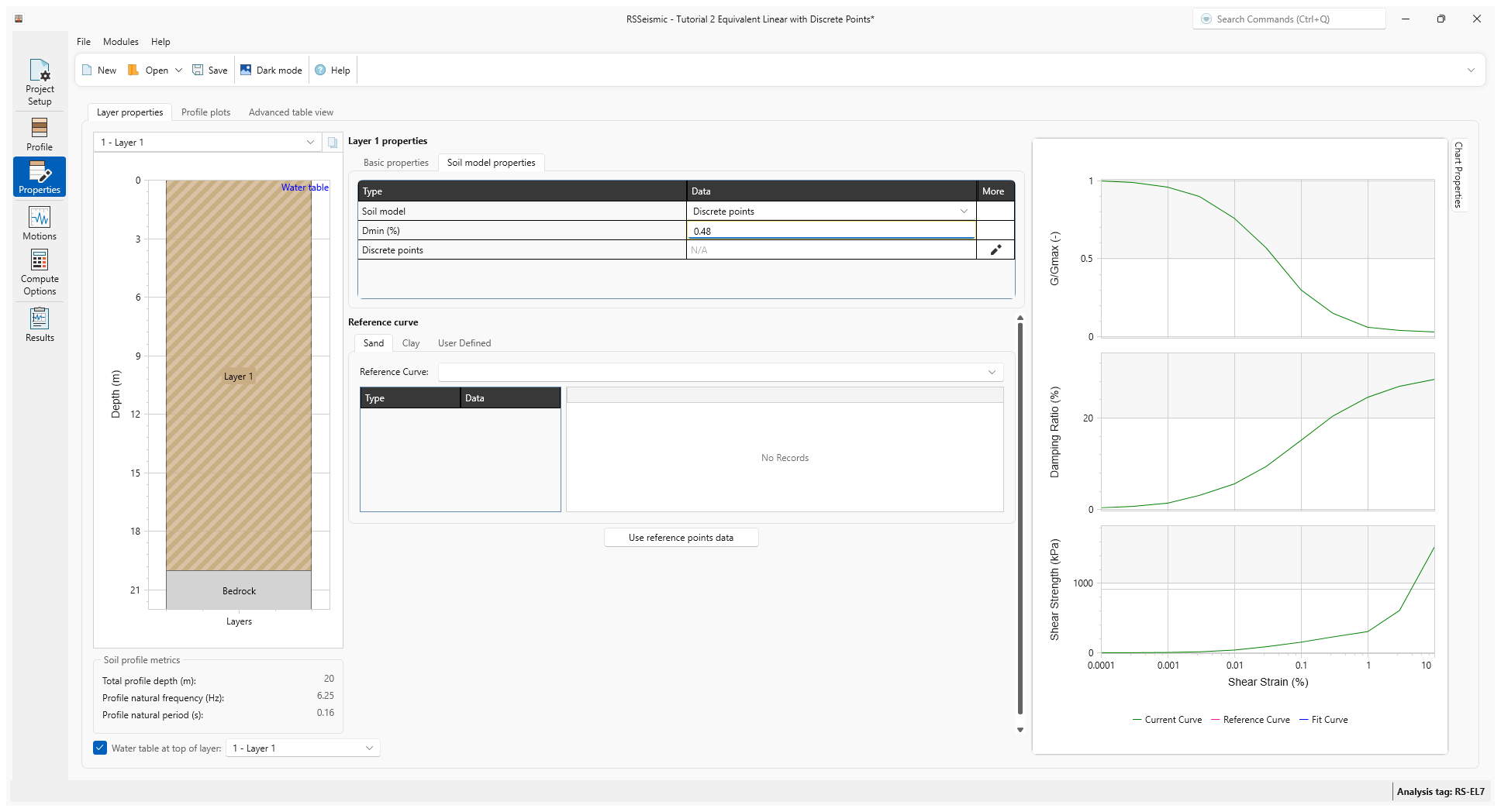
Notice that the current curve on the chart has been updated.

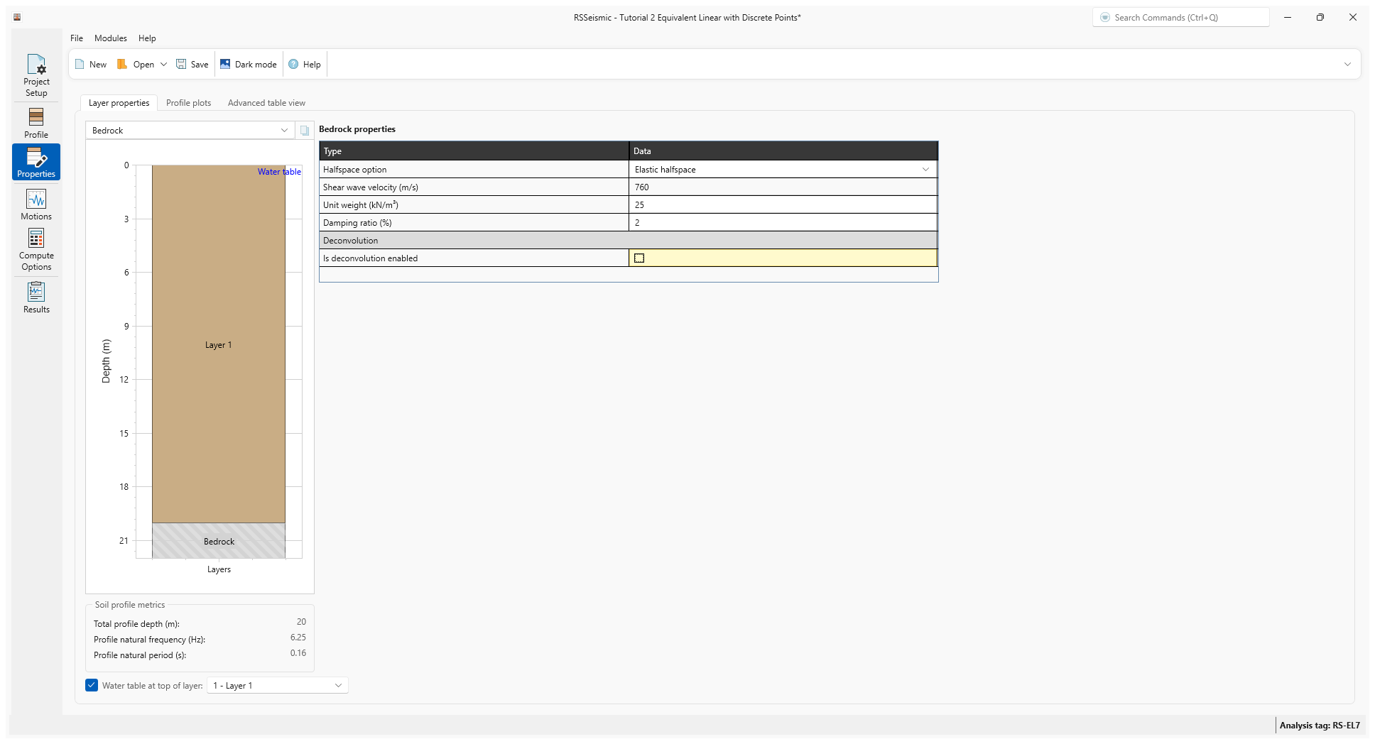
5. Select the Bedrock layer. This can be done either by clicking on the layer in the soil profile diagram (on the left) or using the drop down list at the top left of the Layer Properties tab.
6. Under Bedrock Properties, set the Halfspace option to Elastic halfspace.
7. Enter the following:
   1. Shear wave velocity (m/s) = 760
   2. Unit weight (kN/m³) = 25.0
   3. Damping Ratio (%) = 2.0

5.0 Motions

1. Go to the Motions tab
   

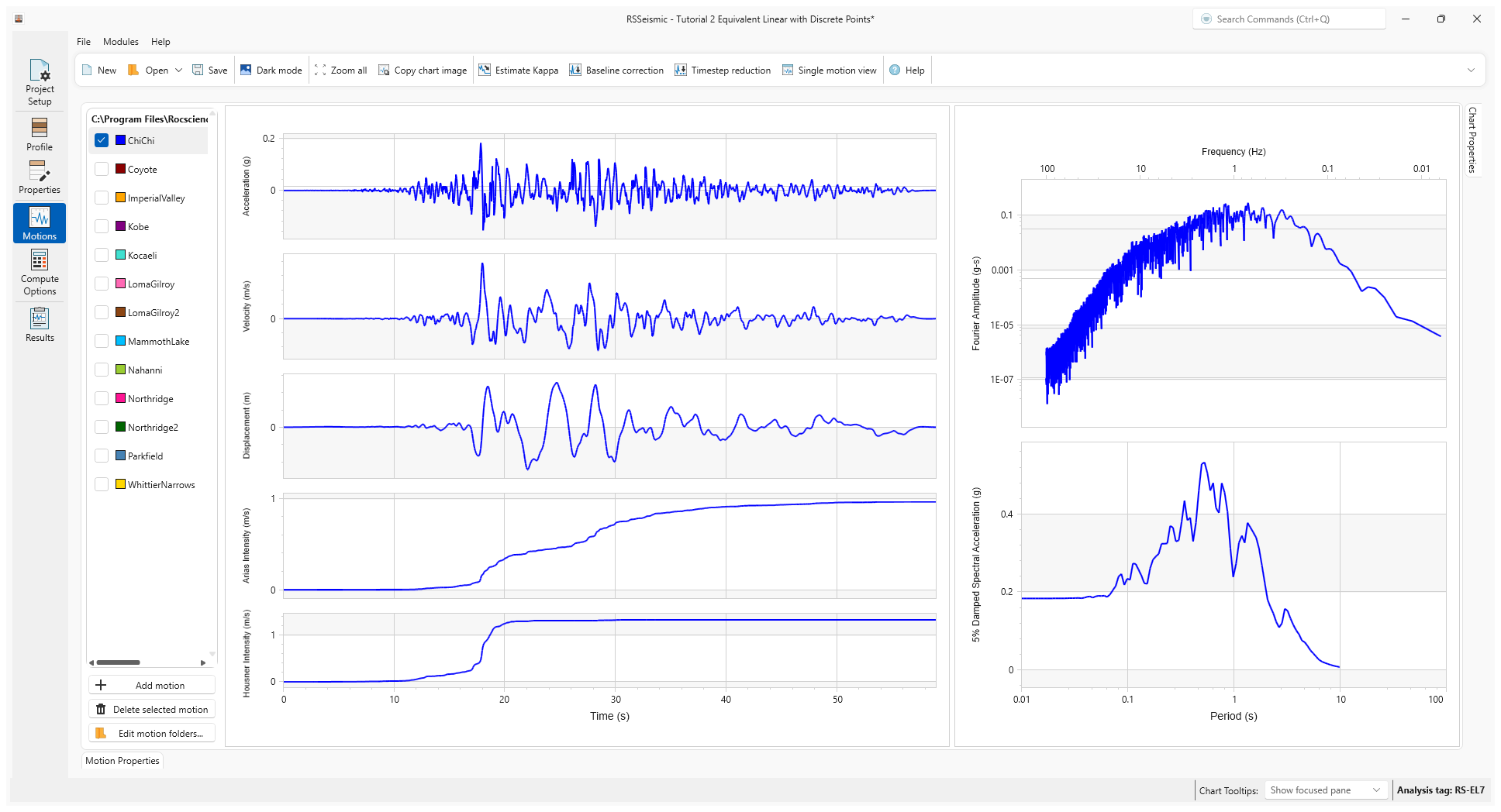
The Motions tab is used to view/process input motions. RSSeismic will generate acceleration, velocity, displacement and Arias intensity time histories, as well as the response spectrum and Fourier amplitude spectrum for the selected motion.

For this tutorial, we will select the ChiChi motion.

2. Under Resources/Input Motions, tick the checkbox for ChiChi.

The time-history (Acceleration, velocity, displacement, Arias and Housner Intensity) and spectral plots (5% damped spectral acceleration) and Fourier Amplitude Spectrum (FAS) of selected the motion can be viewed.

6.0 Compute

1. Go to the Compute Options tab
   

The Compute Options tab provides the user with the ability to control some aspects of the numerical solution scheme.

Since we have selected a Frequency Domain solution, only the Frequency Domain options will be available.

2. Under Frequency Domain ensure the following values are selected:
   1. Number of iterations = 15
   2. Effective Shear Strain Ration = 0.65
   3. Complex Shear Modulus Formulation = Frequency Independent (recommended)
3. For Output Settings, leave the default Layers = Surface Only. Output Displacement Animation should also be turned ON by default.
4. Click Compute.
5. Once the compute is complete, click Save to save your project.

7.0 Results

1. Go to the Results tab
   

The Results section of RSSeismic contains a series of tabs to that allow you to review the results of your analysis.

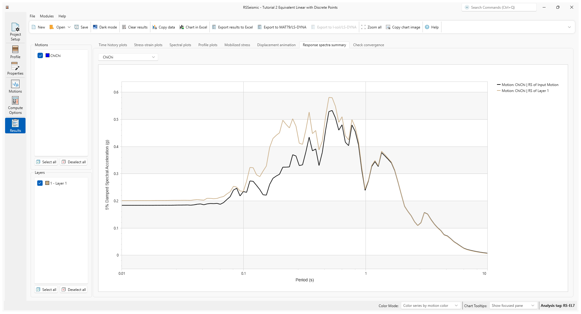
Below are the computed time-histories (Acceleration, Velocity, Displacement, and Arias Intensity) and response spectrum at the first layer of the site profile along with that of input motion.

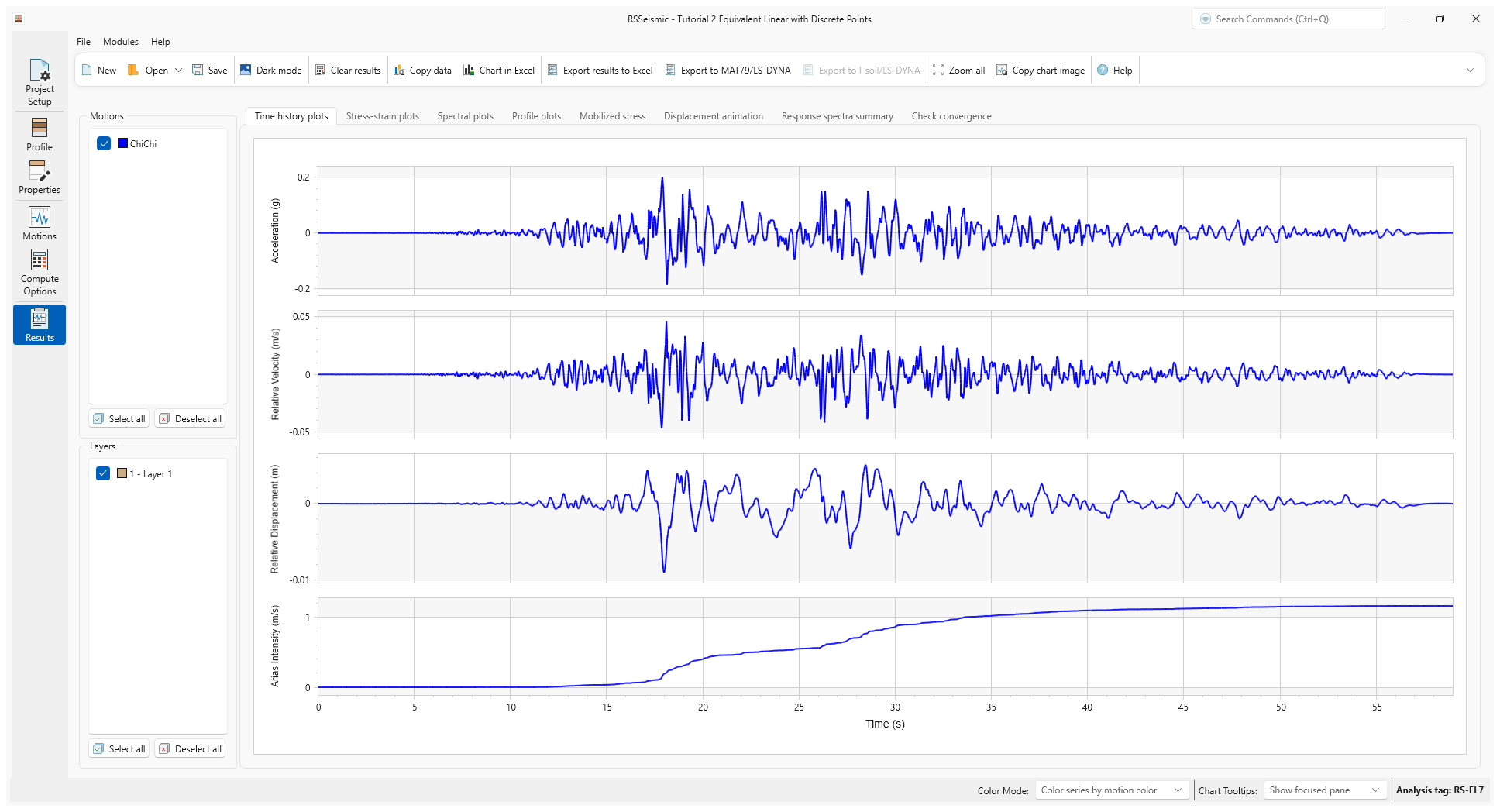
The response spectra plot shows the surface and input motion spectra allowing the user to examine how the soil column modified the ground motion. In this example, the soil column amplified the ground motion for a period less than about 0.8 sec.

8.0 Additional Exercise: Multiple Layers

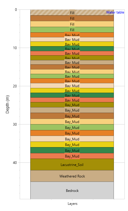
San Francisco Bay Mud soil profile

1. Select File > Recent Folders > Tutorial Folders and go to the Tutorial 2 folder.
2. Open the file Tutorial 2 Bay Mud Profile.

Similar to the example we just did, this is an example of an Equivalent Linear Frequency Domain analysis with Discrete Points, but this soil profile includes 31 layers instead of just 1 (shown below). This is a typical soil profile near San Francisco Bay, and is included to illustrate the capabilities of RSSeismic for more realistic soil profiles.

8.1 Properties

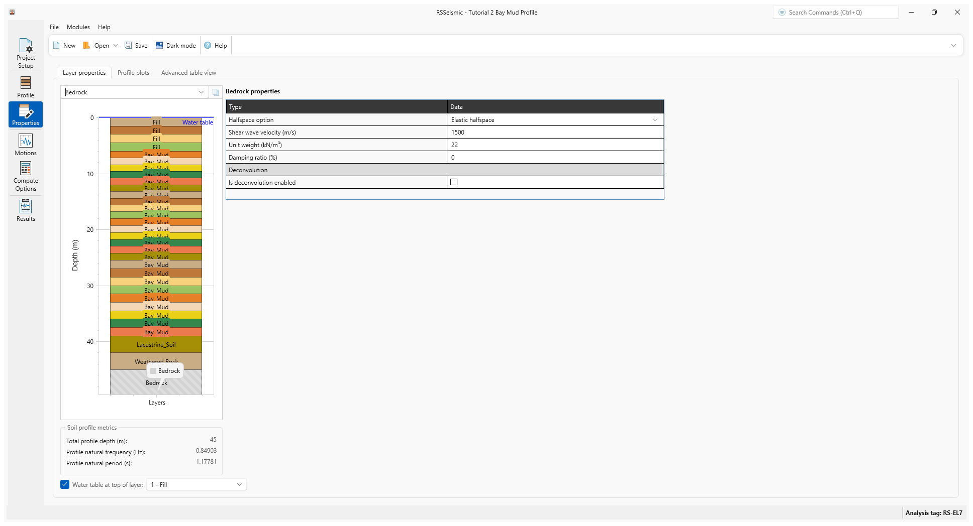
1. Go to the Properties tab .
   Notice the soil profile parameters and discrete points have been defined for each layer. They represent the dynamic properties for the corresponding fill and Bay Mud layers.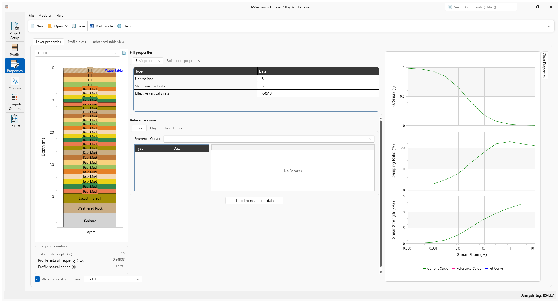
   
2. Select the Advanced table view to review all the layer properties at once.
   
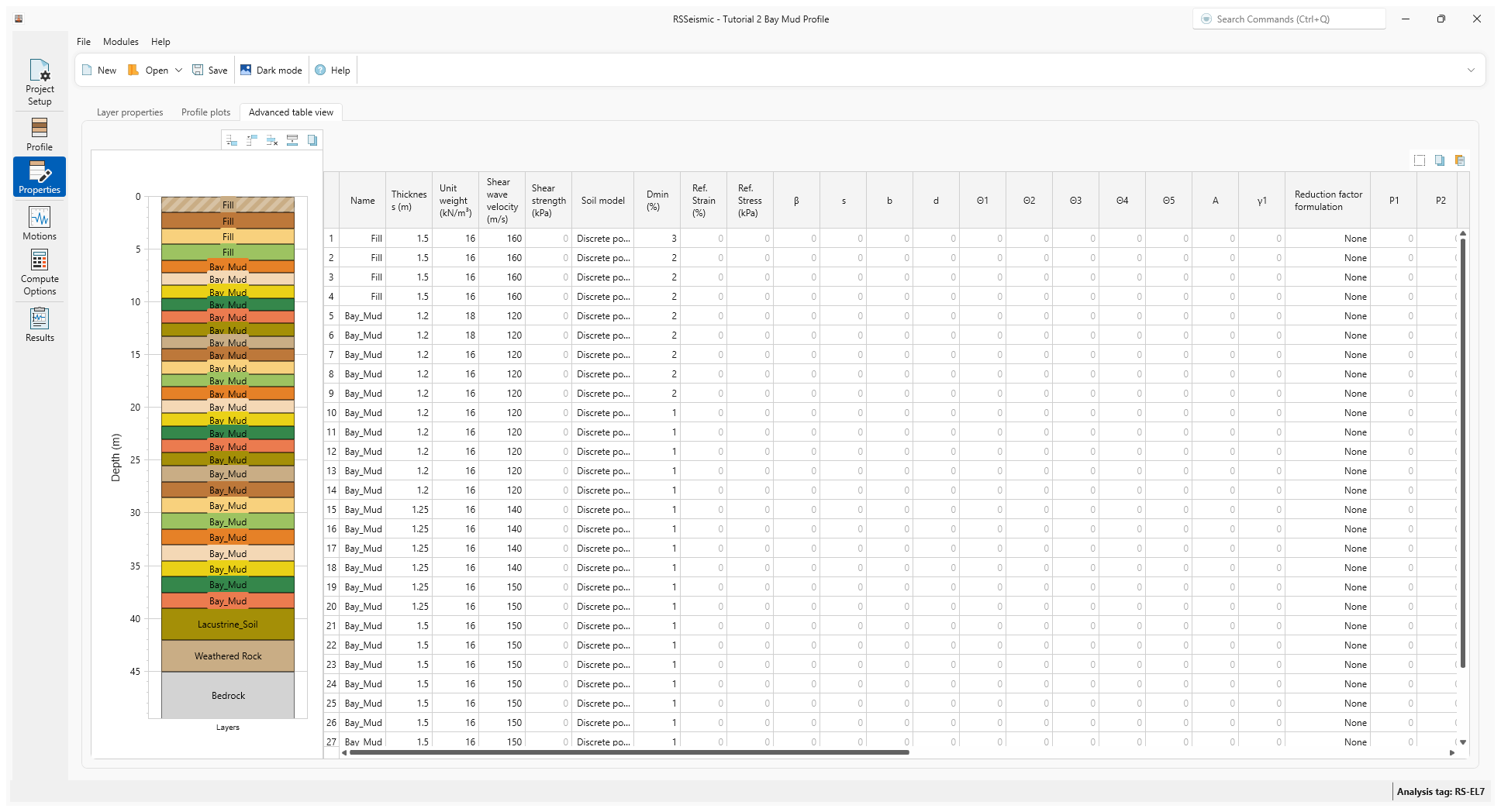
3. If you return to the Layer Properties and select the Bedrock layer, you can see it is defined as elastic halfspace with a shear wave velocity of 1500 m/s, unit weight of 22 kN/m³ and damping ratio of 0.0%.
   

8.2 Motions

1. Go to the Motions tab .
2. Under Resources\Input Motions, ensure ChiChi is selected.

8.3 Compute Options

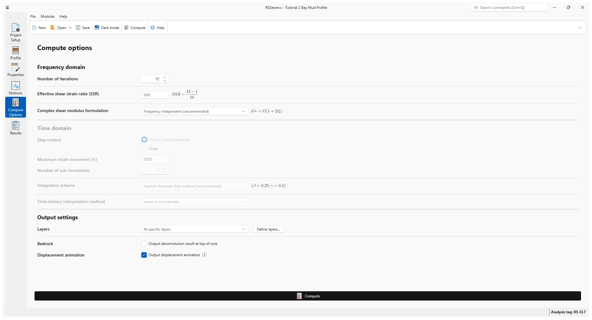
1. Go to the Compute Options tab .
2. We will use the default options for Frequency Domain (as we did in the previous model).
3. For the Output Settings, we will be computing one layer, but this time we will select one of the middle layers in the soil profile.
   1. Select Layers > At specific layers.
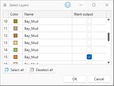
   2. Click Define to open the select layers dialog.
   3. Click Deselect All and then select layer 15 – Bay Mud.
   4. Click OK.
      
4. Click Compute.
5. Once the project is computed, click Save .

8.4 Results

1. Go to the Results tab .
2. Below are the computed Time History Plots (accelertion, velocity, displacement and Arias intensity).
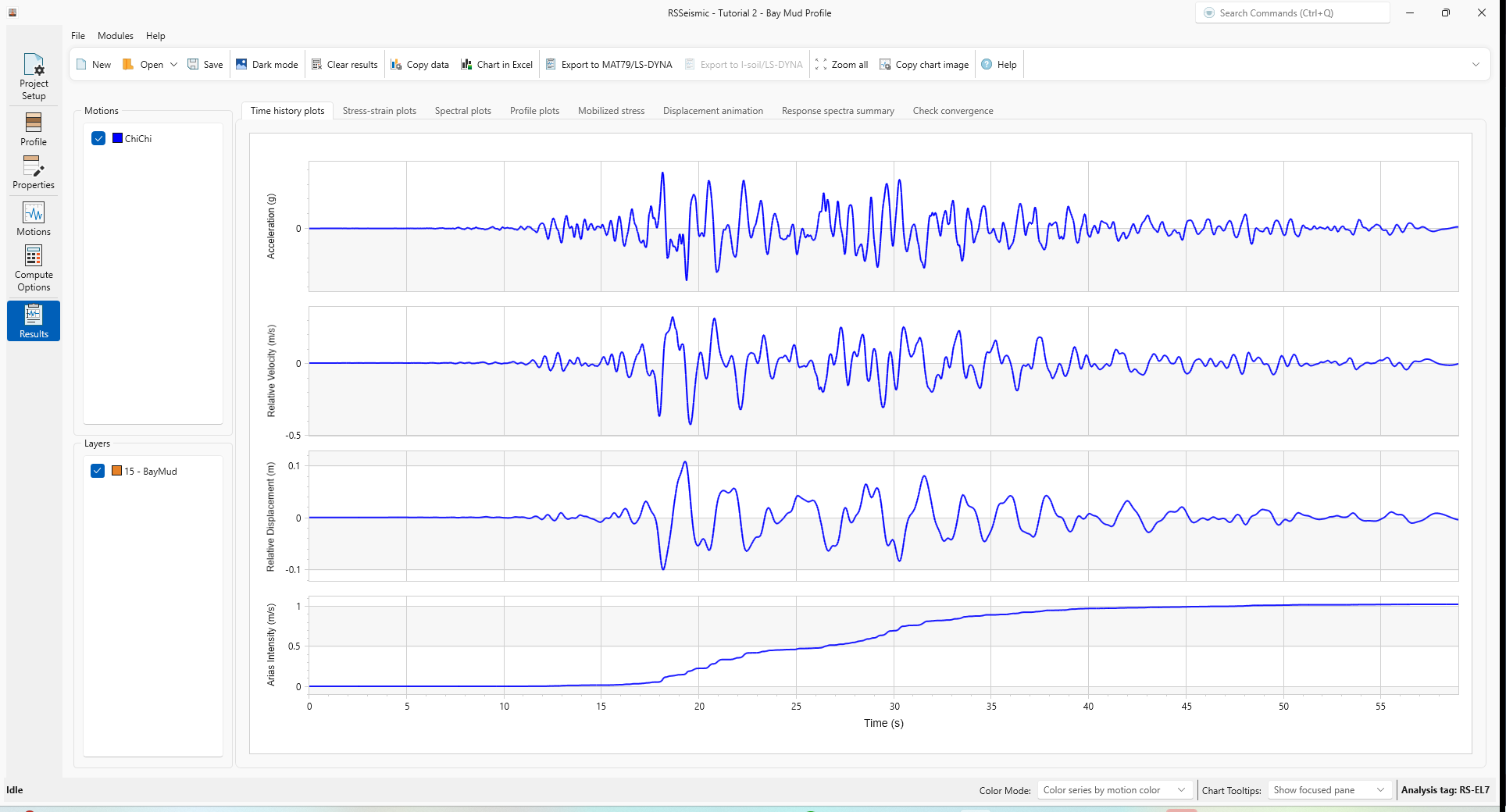
3. Select the Profile Plots tab.
   
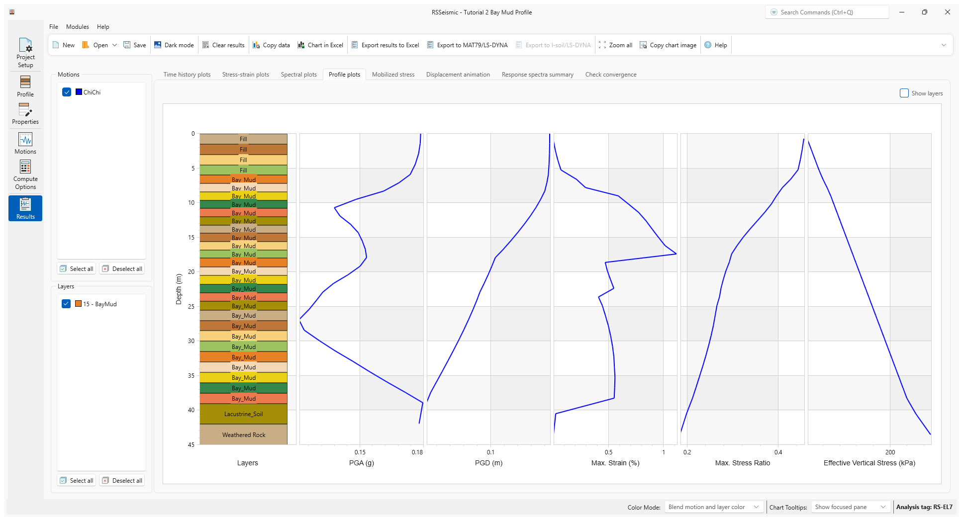
   The profile plots show the variation of various parameters as the ground motion is propagated through the soil profile. For example, the maximum strain profile shows the level of strains experienced in the various layers.
   
4. Select the Response Spectra Summary tab.
   

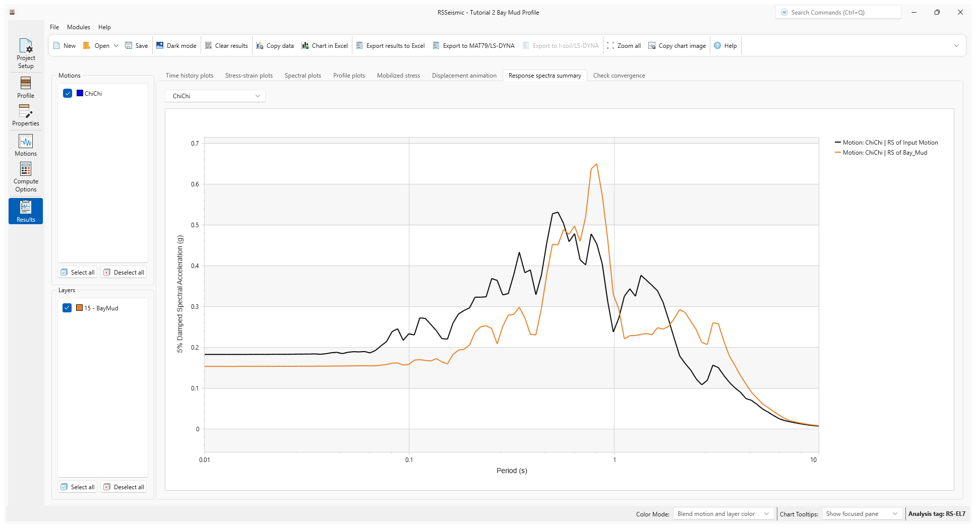
The response spectra plots show the impact of the soil column on the propagated ground motion. The ground motion at low period (below~0.8 sec) is attenuated while the ground motion at the larger period is significantly amplified. This is expected for soft soil columns and is consistent with field observations.