3 - Nonlinear and Equivalent Linear Analysis

1.0 Introduction

This tutorial consists of a nonlinear site response analysis, along with a supplementary equivalent-linear analysis. The GQ/H model with non-masing type of re/unloading formulation is used for soil dynamic curves. This is used in conjunction with a frequency independent small strain damping formulation and an elastic bedrock.

This tutorial will guide the user through the most commonly used analysis options encountered when performing a single profile site response analysis:

1. Nonlinear analysis with equivalent linear analysis results option: This feature in RSSeismic allows the user to prepare a streamlined single input work-flow while providing analysis results using both the nonlinear, time-domain, and equivalent linear, frequency-domain, analysis procedures. Commonly, users have to use two separate analysis platforms to obtain both results, having to learn two different input processes, and incurring significant cost. The user is then faced with a choice of trying to select which analysis procedure to use, with apriori being able to decide if it is an appropriate choice. Having both results also allows the user to quickly identify potentially unique issues with the profile that might need to be carefully examined.
2. Ground motion: The ground motion of interest is an outcrop motion. This is what seismic hazard analysis provides, or a motion that is fitted to a target response spectrum. Hence an elastic bedrock option is used.
3. GQH model with non-masing reloading/unloading: This soil model fits the target dynamic curves, while at the same time being constrained by the soil strength at large strain. The non-masing unloading/reloading formulation allows the user to fit the damping curves commonly available and are based on laboratory test. Otherwise, if masing rules are used, material damping in the soil layers would be greatly overestimated. The model generates fitted dynamic curves when used in equivalent linear frequency domain analysis and represents the cyclic behavior of soil when used in nonlinear time domain analysis.
4. For small strain damping in nonlinear domain a frequency independent formulation is used. This overcomes the severe limitations of Rayleigh damping, which leads to a numerical artifact of frequency dependent damping leading to under or over estimation of the damping depending on the frequency range, used in many implementations, and obviates the need to identify the target frequencies to be used.

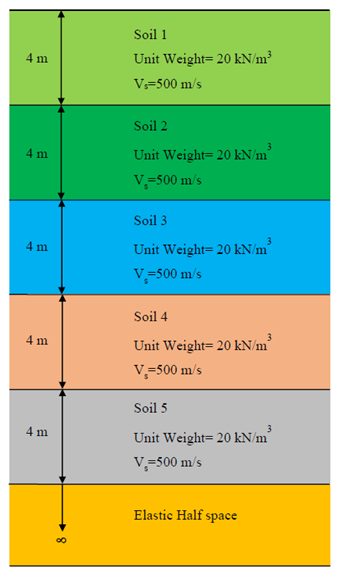
The example soil profile consists of 5 layers, 4 m each, with a bedrock layer (also termed reference rock condition) defined as elastic halfspace.

Topics covered in this tutorial:

• Nonlinear Time Domain Analysis
• Equivalent Linear Frequency Domain Analysis
• Dynamic Curve Fitting

Finished Product:

The finished product of this tutorial can be found in the Tutorial 3 folder. All tutorial files installed with RSSeismic can be accessed by selecting File > Recent Folders > Tutorials Folder from the RSSeismic main menu.

2.0 Project Setup

1. Begin by opening the RSSeismic program and selecting New Project . A new project will open, and you will be taken to the Project Setup tab.
2. Before proceeding with the project parameters, save your project. Select File > Save Project and save your project as Tutorial 3 Nonlinear and Equivalent Linear Analysis.
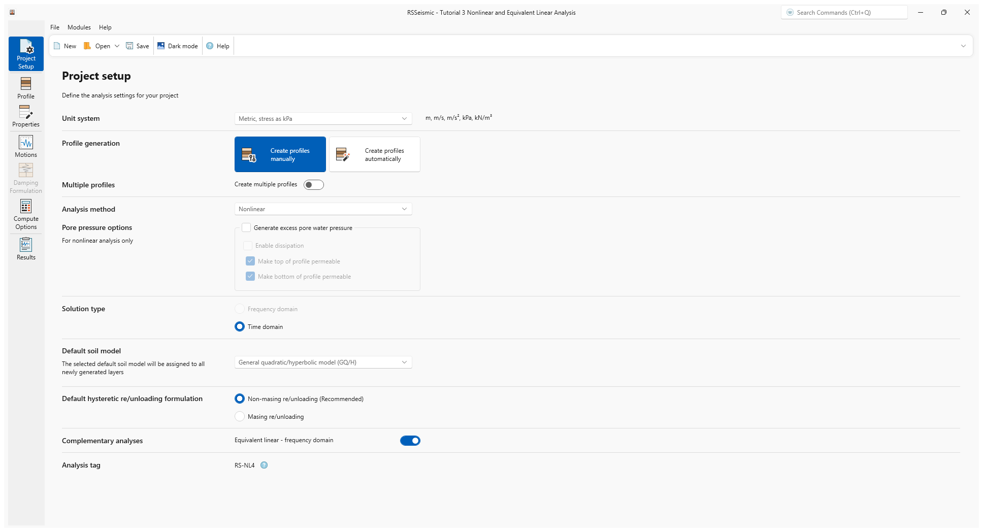
3. In the Project Setup tab, set the Unit System to Metric, stress as kPa.
4. For the Profile Generation, we will be leaving the default: Create Profiles Manually. Since we are only defining one soil profile, Create Multiple Profiles will remain turned off. (See the Profiles topic for details on creating multiple profiles.)
5. For Analysis Method select Nonlinear. Leave all Pore pressure options turned OFF.
6. The Solution type will be set to Time Domain by default.
7. For Default Soil Model, ensure General quadratic/hyperbolic model (GQ/H) is selected.
8. For Default hysteretic re/unloading formulation ensure the default Non-masing re/unloading (recommended) is selected.

When conducting a Nonlinear analysis, users have the option of obtaining the site response results using the Equivalent Linear method automatically. This can be done by using the Complementary analyses option. We will be using this option for the tutorial.

9. For Complementary analyses, ensure Equivalent Linear – Frequency Domain is selected.

3.0 Profile

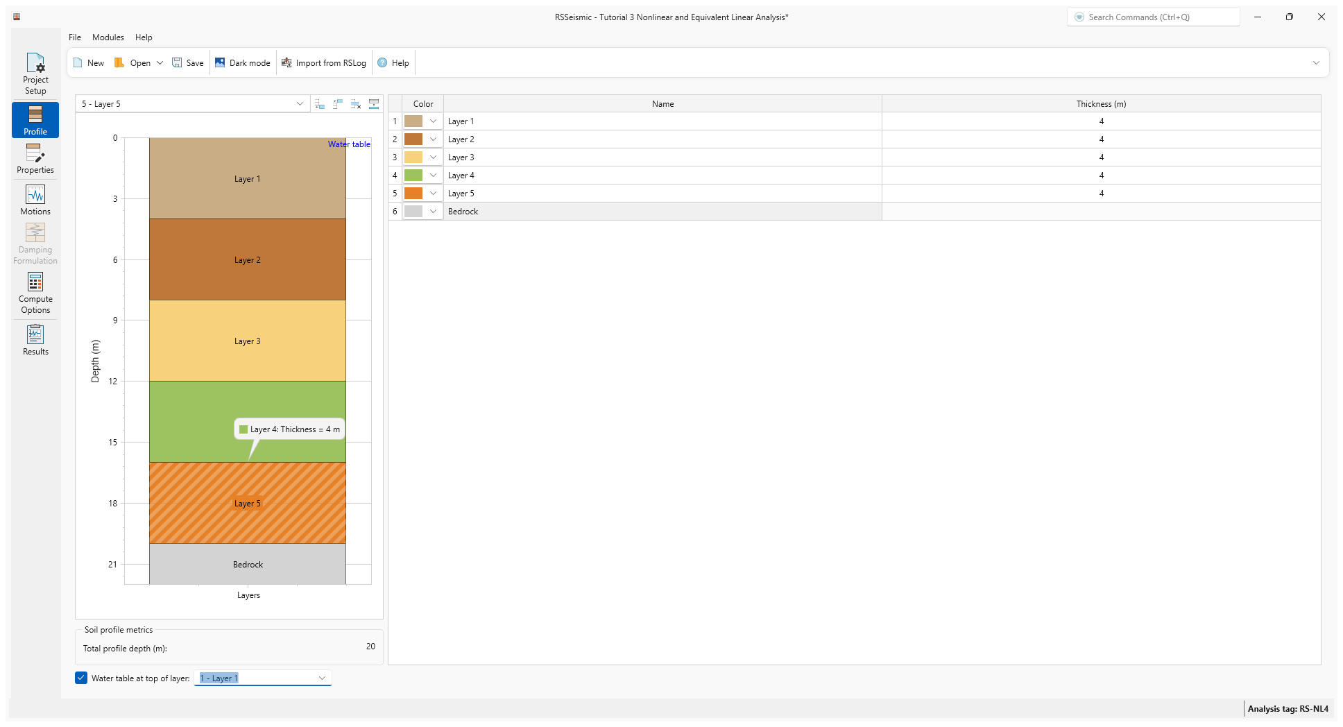
1. Go the Profile tab
   

For this tutorial, we will be creating a soil profile with a total of 5 soil layers.

2. Add 4 more layers to the soil profile. This can be done by clicking Add Layer Below 4 times, or by clicking Append Rows and entering 4. You should now have 5 layers total.
3. Change the Thickness of each layer to 4 m.
4. Tick the Water table at top of layer checkbox to add a water table above Layer 1. This implies that the ground water table is at the ground surface.

4.0 Properties

1. Go to the Properties tab
   

Layer 1 will be selected by default.

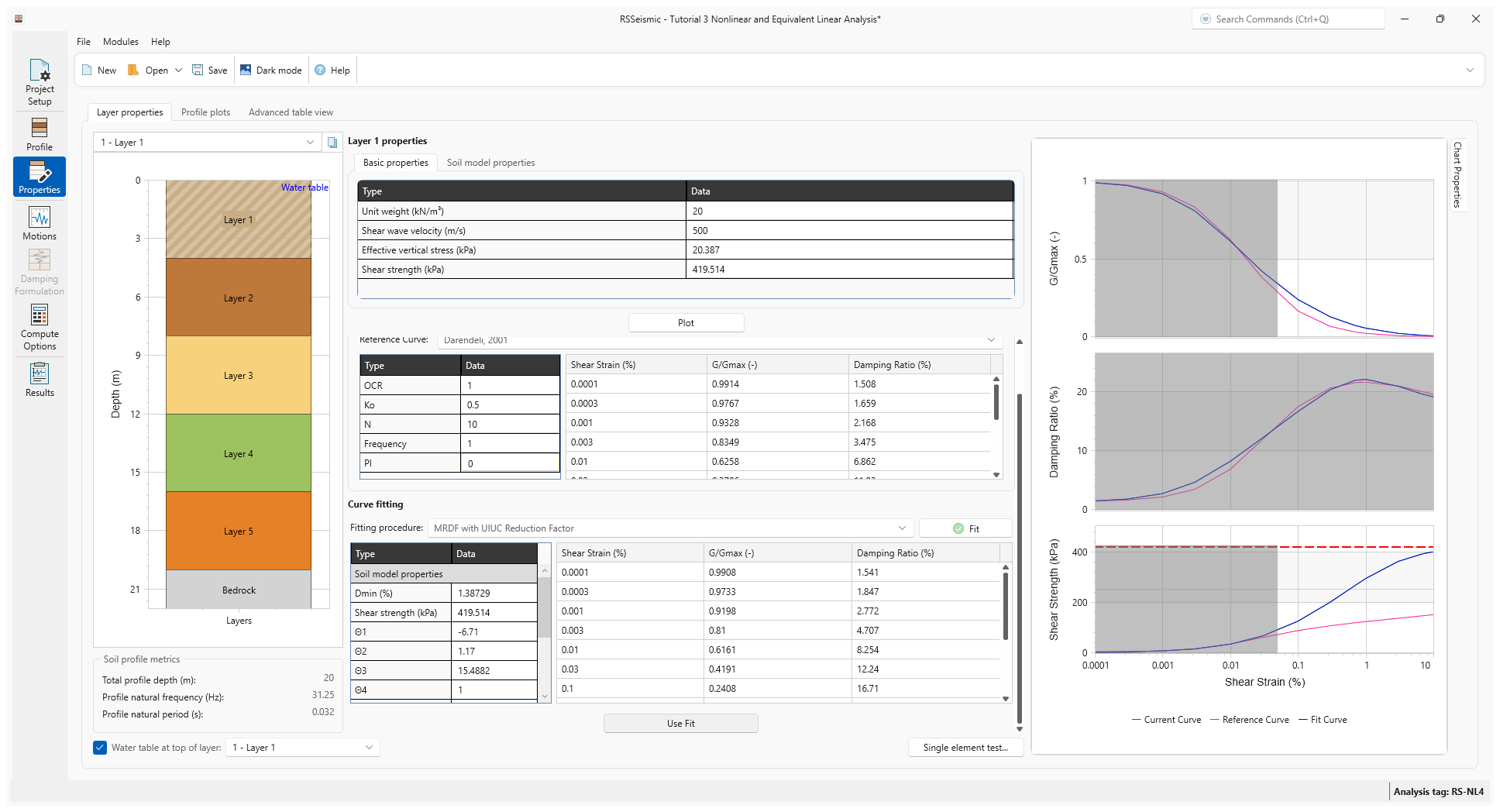
2. Under Basic Properties enter:
   1. Unit Weight (kN/m³) = 20
   2. Shear wave velocity (m/s) = 500
   3. Effective vertical stress (kPa) = 20.38
   4. Shear strength (kPa) = 419.514
3. Under Reference Curve > Sand select the Darendeli, 2001 reference curve.

A library of curves, extracted from the published literature is available for the user to select from. In this example we use one of the most commonly used set of curves, Darendeli (2001). The user can choose other available curves if they better represent the characteristics of the site of interest, or input their own curves.

4. Enter Ko = 0.5. Leave all others values as the defaults shown below:
   1. OCR = 1
   2. Ko = 0.5
   3. N = 10
   4. Frequency = 1
   5. PI = 0
5. Under Curve Fitting, enter Fitting Procedure = MRDF with UIUC Reduction Factor.

The UIUC Reduction factor does not allow for the damping to reduce in value at large strains. The alternative would allow for this reduction to occur as proposed in the original Darandeli formulation.

6. Click Fit.
7. The Fitting Limits dialog will appear. Leave the default values (Max strain = 0.05% and Min Strength = 95%) selected and click OK.

8. The Soil Model properties and Reduction factor formulation will be calculated. Click Use Fit to apply the fitted curve to Layer 1.

In the resulting fitted curve you will notice that normalized shear modulus reduction curve is matched well up to a strain of about 0.1 %. Beyond that the fitted curve in stress-strain space climbs to approach the target shear strength. The implied strength in the target curve is significantly less than the target soil strength and hence the necessity for this departure. The damping curve is well matched for the full strain range.

9. Repeat Steps 3-8 above for Layers 2-5. Use the basic properties listed in the table below to develop the fitted curves and use the corresponding model parameters.

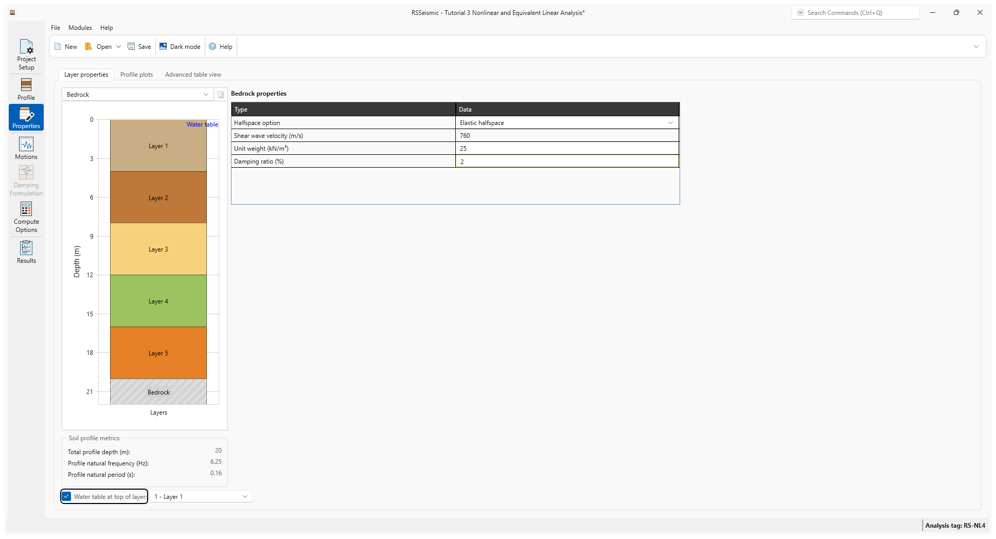
10. After completing the curve fitting for all the soil layers, select the Bedrock layer. Enter:
    1. Halfspace option = Elastic Halfspace
    2. Shear wave velocity (m/s) = 760
    3. Unit Weight (kN/m³) = 25
    4. Damping ratio (%) = 2
       

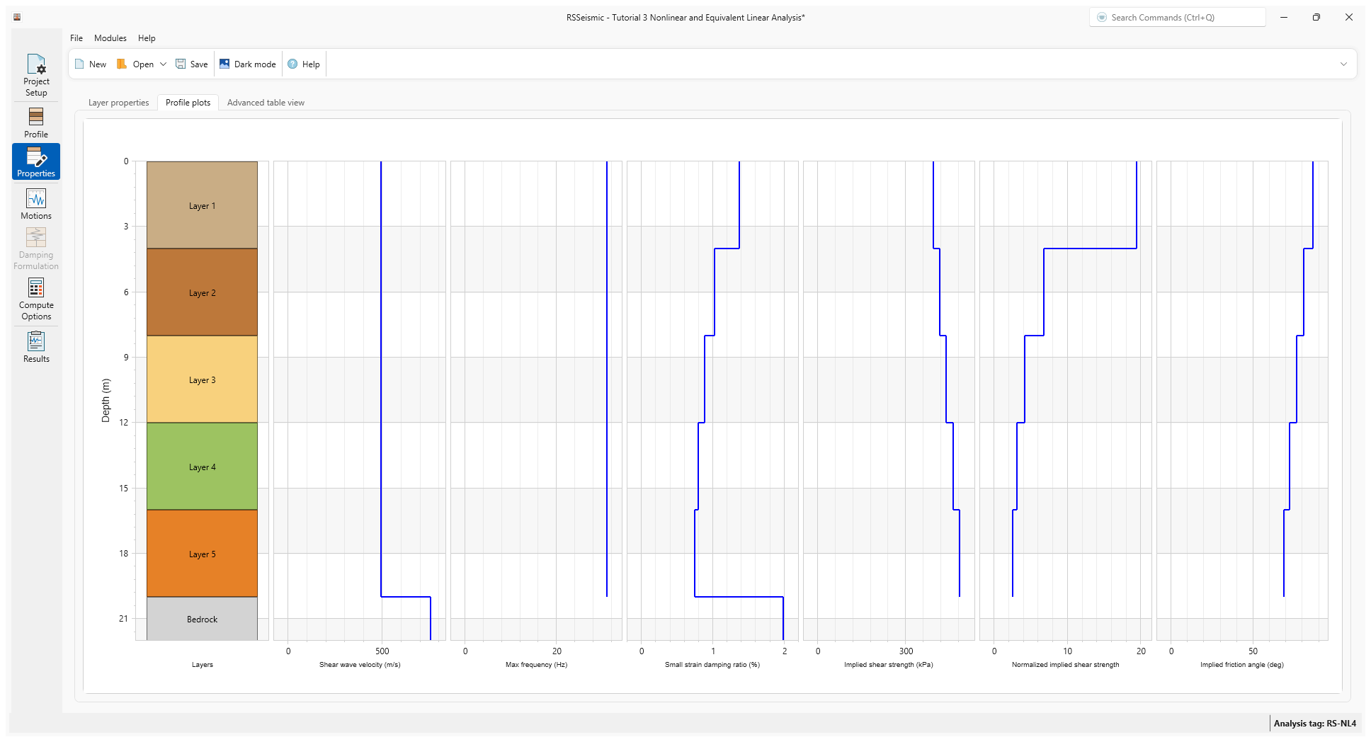
11. Select the Profile Plots tab to review your data.

The user is encouraged to carefully examine these graphs to confirm that the input of selected profile characteristics are as intended. This includes shear wave velocity, the maximum frequency that can be propagated through the soil profile and implied strength properties.

5.0 Motions

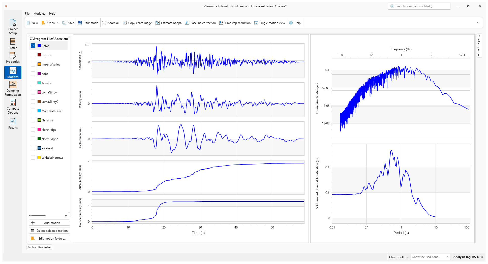
1. Select the Motions tab
   
2. Under Resources\Input Motions, select ChiChi.

6.0 Damping Formulation

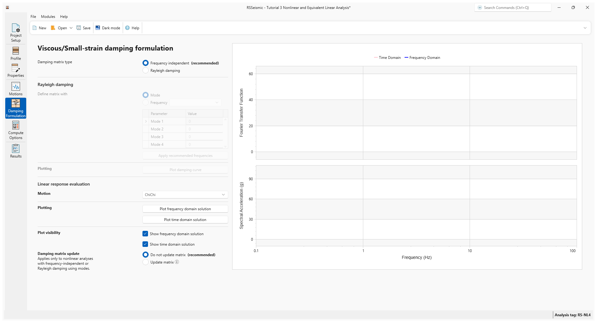
1. Select the Damping Formulation tab
   
2. For Damping Matrix Type we will use the default selection of Frequency Independent.
3. For Damping matrix update, use the default Do not update matrix.

7.0 Compute Options

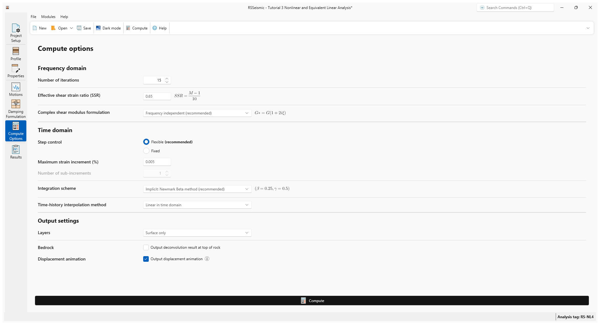
1. Go to the Compute Options tab
   
2. For Frequency Domain use the default values:
   1. Number of iterations =15
   2. Effective Shear Strain Ratio (SSR) = 0.65
   3. Complex Shear Modulus Formulation = Frequency-Independent
3. For the nonlinear Time Domain analysis use the default values:
   1. Step Control = Flexible
   2. Maximum Strain Increment (%) = 0.005 %
   3. Integration scheme = Implicit = Newmark Beta Method
   4. Time History Interpolation Method = Linear in time domain
4. For Output settings ensure Layers = Surface only is selected.
5. Click Compute.
6. After the compute is completed, click Save
   

8.0 Results

1. Go to the Results tab
2. Change the Color Mode to Blend motion and layer color to more easily see the lines.
3. The Time History Plots should look as follows.

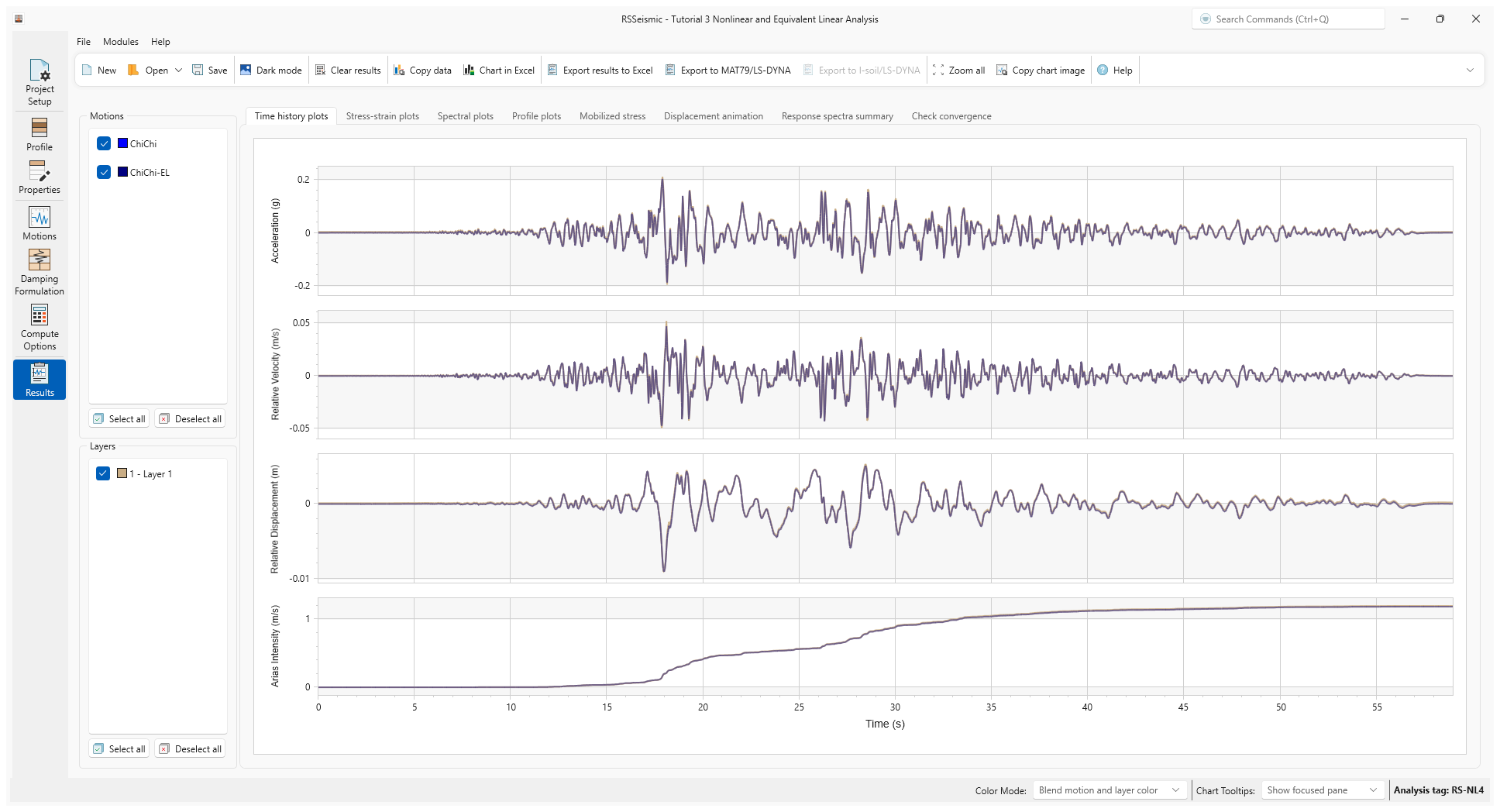
The results tab offers the user several options to view and export the results of the analyses either individually or of multiple analyses. The user is encouraged to examine the computed surface motions (acceleration, velocity and displacement) in addition to surface response and fourier spectra. The user can also examine the stress and strain histories in a selected layer.

3. Select the Profile Plots tab.

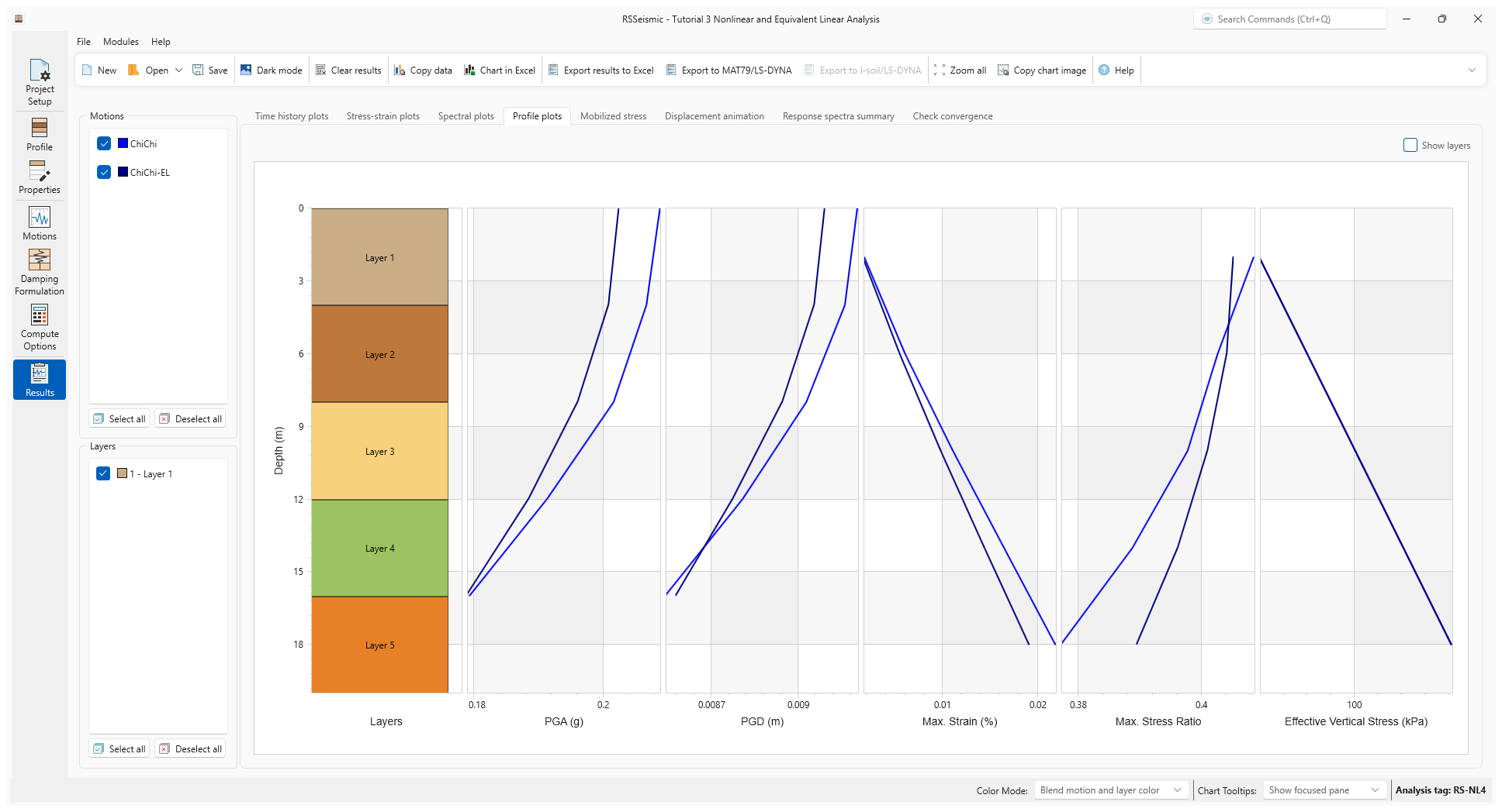
The profile plots show the variation of various parameters as the ground motion is propagated through the soil profile. For example, the maximum strain profile shows the level of strains experienced in the various layers.

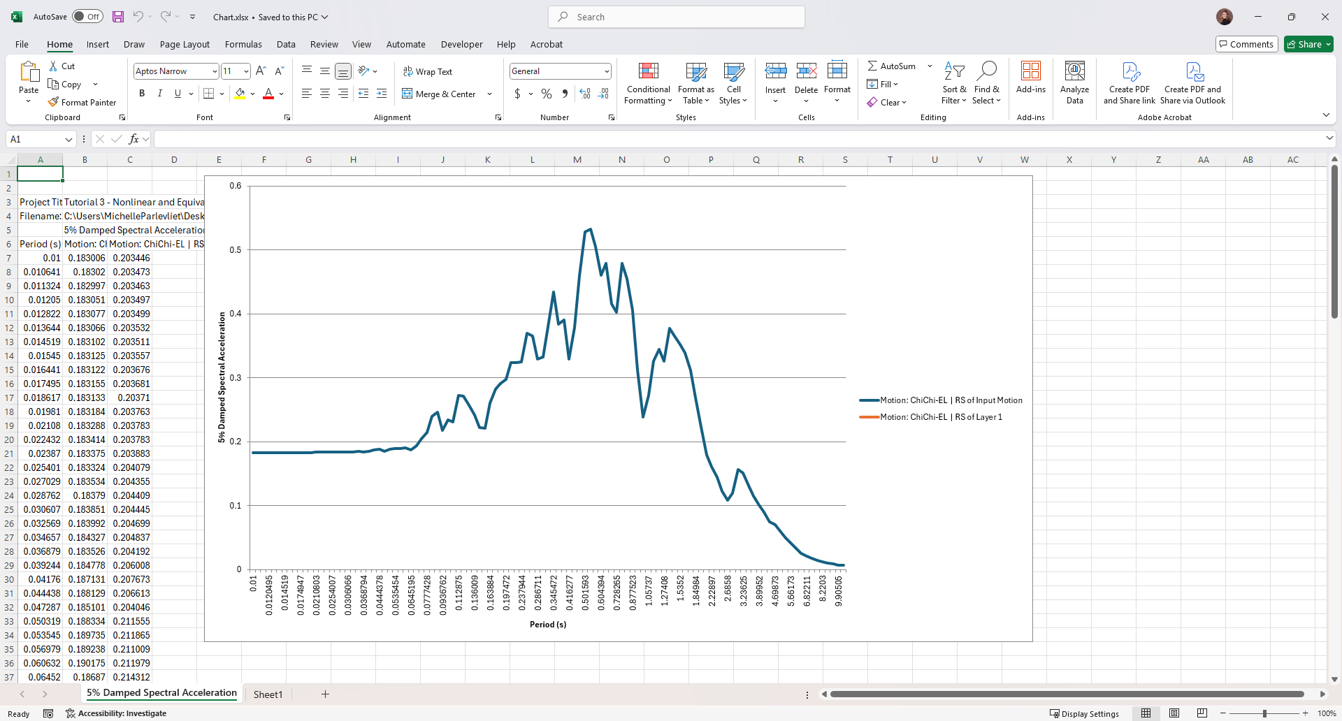
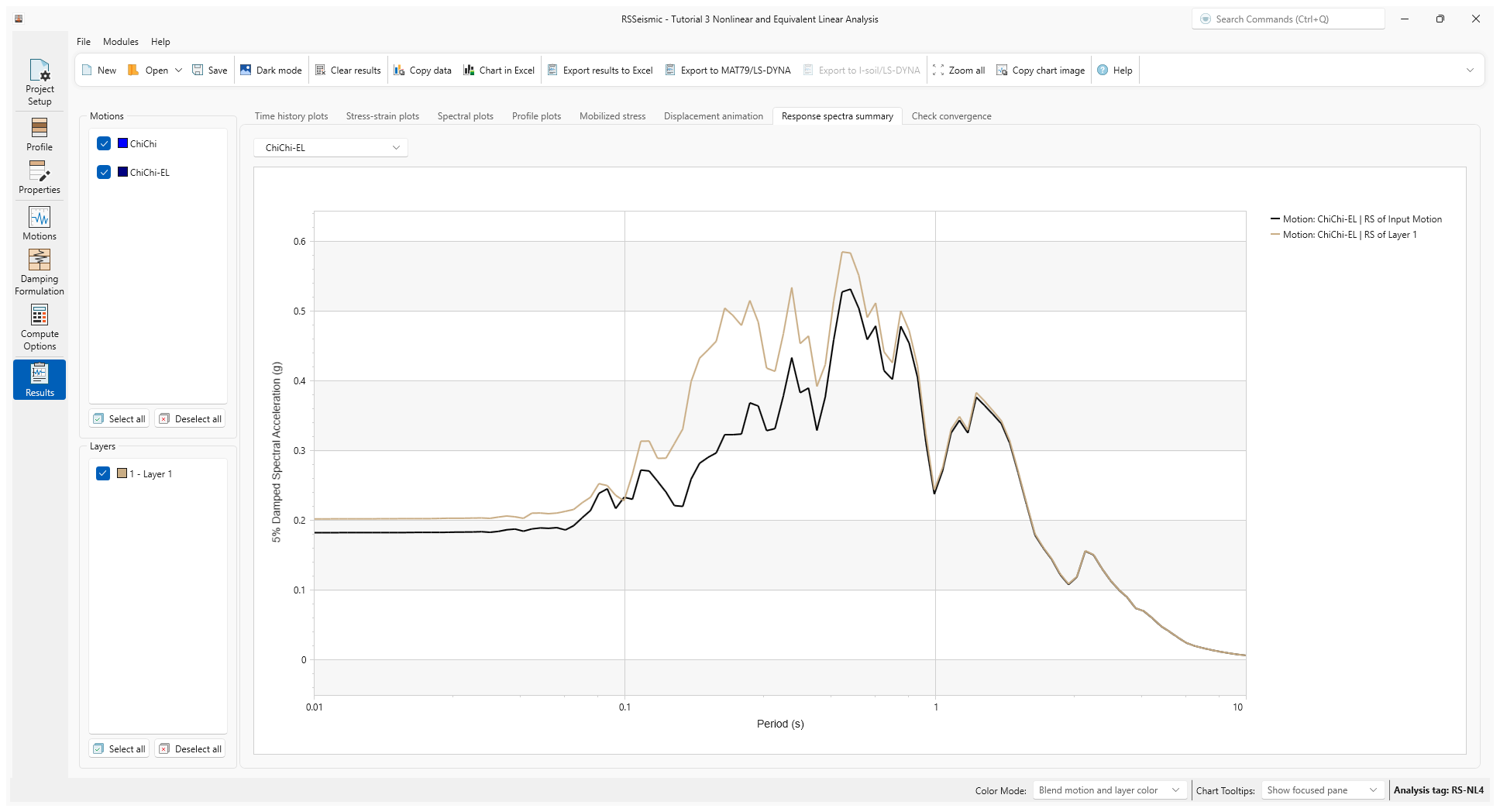
4. Select the Response Spectra Summary tab.

This plot shows the response spectra of both the input motion and the computed surface motion. The user can thus view how the ground motion is amplified or attenuated by the soil profile.

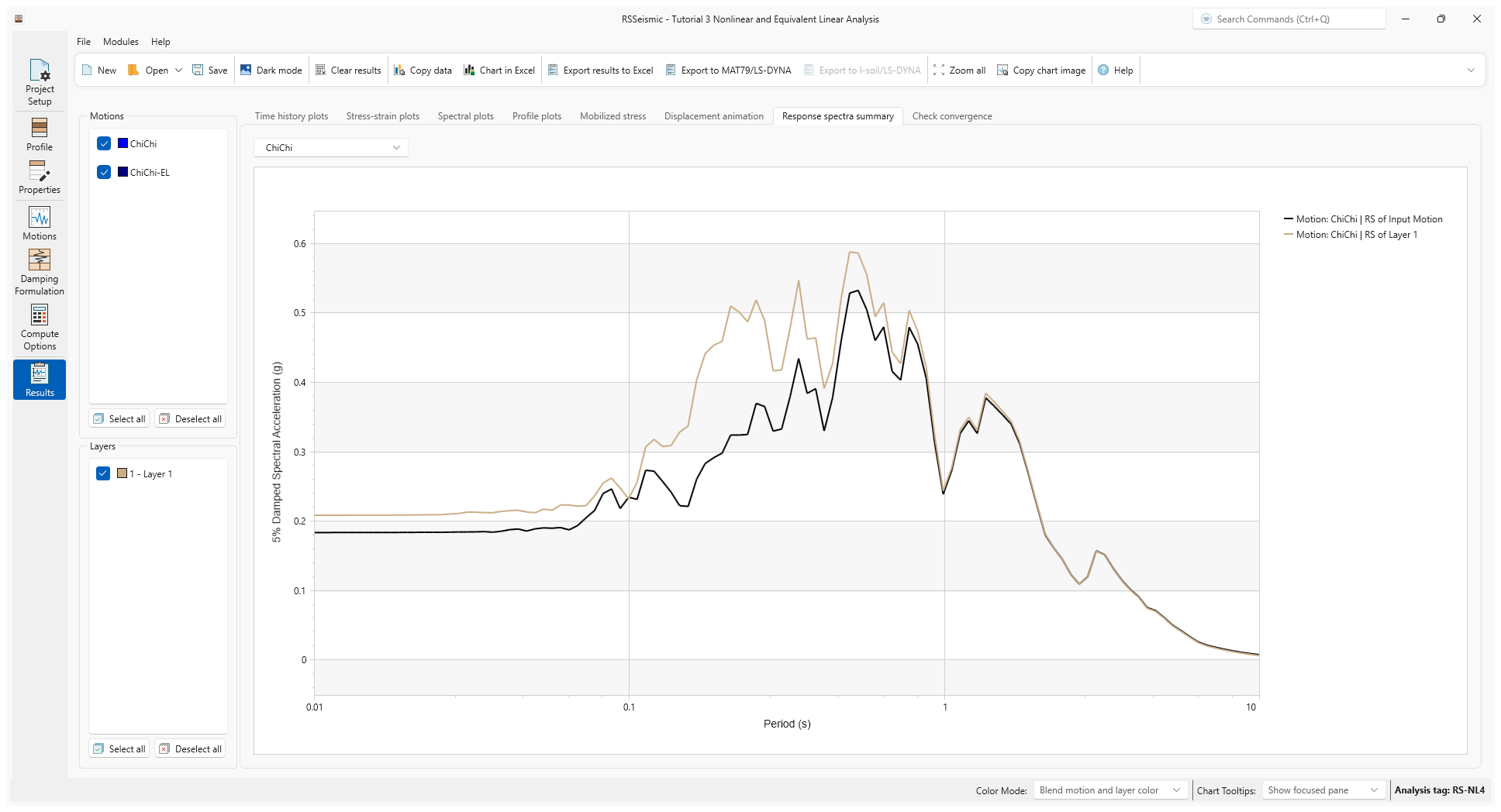
5. Use the Motion drop down to compare the ChiChi motion to the ChiChi-EL results.

6. The results the analysis can be exported to a spreadsheet using the Export to Excel option. Click Chart in Excel in the toolbar, select a name and location for the file, and click Save. The Excel sheet will open automatically.