8 – Nonlinear Analysis with Finite Element Engine
1.0 Introduction
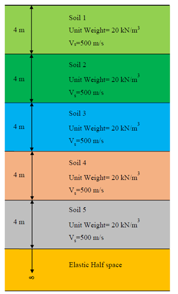
This tutorial consists of a nonlinear site response analysis using the finite element engine, along with complementary equivalent linear and nonlinear analyses using the lumped mass engine. The I-soil and GQ/H constitutive models are used to model the soil response in the finite element and lumped mass analyses, respectively. This tutorial uses the same soil profile as Tutorial 3.
Topics Covered in this Tutorial:
- Nonlinear time domain analysis with FEM engine
- Complementary equivalent linear and nonlinear lumped mass analyses
- Dynamic curve fitting
Finished Product:
The finished product of this tutorial can be found in the Tutorial 8 folder. All tutorial files installed with RSSeismic can be accessed by selecting File > Recent Files/Folders > Tutorials Folder from the RSSeismic main menu.
2.0 Project Setup
- Begin by opening RSSeismic and selecting New Project
 . A new project will open, and you will be taken to the Project Setup tab.
 - Before proceeding with the project parameters, save your project. Select File > Save Project
 and save your project as Tutorial 8 Nonlinear FEM Analysis.
 - In the Project Setup
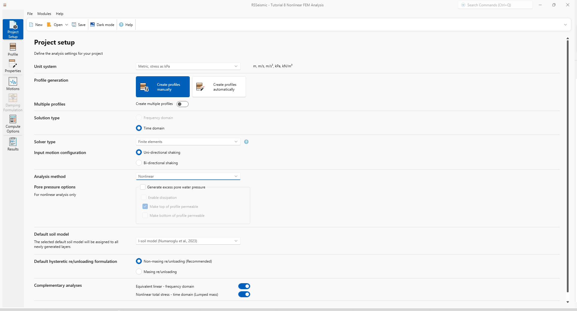
 tab, set the Unit System to Metric, stress as kPa.
 - For the Profile Generation, we will be leaving the default: Create Profiles Manually. Since we are only defining one soil profile, Create Multiple Profiles will remain turned off. (See the Profiles topic for details on creating multiple profiles.)
- For Solution type select Time Domain.
- For Solver type select Finite elements
- For Input motion configuration select Uni-directional shaking
- For Analysis Method select Nonlinear. Leave all Pore pressure options turned OFF.
- For Default Soil Model, ensure I-soil model (Numanoglu et al., 2023) is selected.
- For Default hysteretic re/unloading formulation ensure the default Non-masing re/unloading (recommended) is selected.
When conducting a Nonlinear finite element analysis, you have the option of simultaneously running equivalent linear and nonlinear analyses using the lumped mass engine. This can be done by using the Complementary analyses option. We will be using this option for the tutorial.
- For Complementary analyses, ensure Equivalent Linear – Frequency Domain and Nonlinear total stress – time domain (Lumped mass) are selected.
3.0 Profile
- Go the Profile
 tab.
tab.
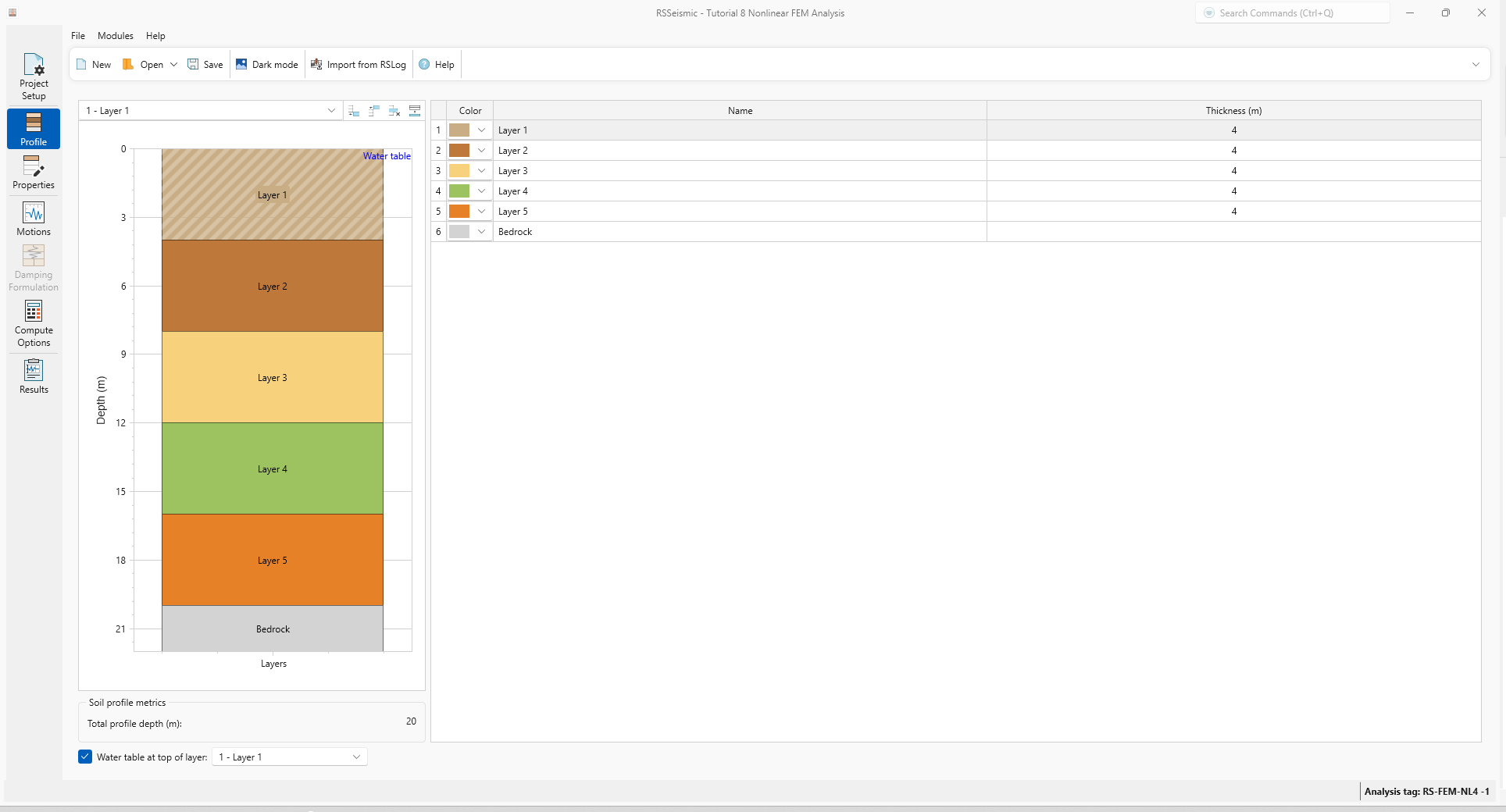
For this tutorial, we will be creating a soil profile with a total of 5 soil layers.
- Add 4 more layers to the soil profile. This can be done by clicking Add Layer Below 4 times, or by clicking Append Rows and entering 4. You should now have 5 layers total.
- Change the Thickness of each layer to 4 m.
- Tick the Water table at top of layer checkbox to add a water table above Layer 1. This implies that the ground water table is at the ground surface.
4.0 Properties
- Go to the Properties
 tab.
tab.
Layer 1 will be selected by default.
- Under Basic Properties enter:
- Unit Weight (kN/m3) = 20
- Shear wave velocity (m/s) = 500
- Effective vertical stress (kPa) = 20.38
- Shear strength (kPa) = 419.514
- K0 = 0.5
- ν = 0.33
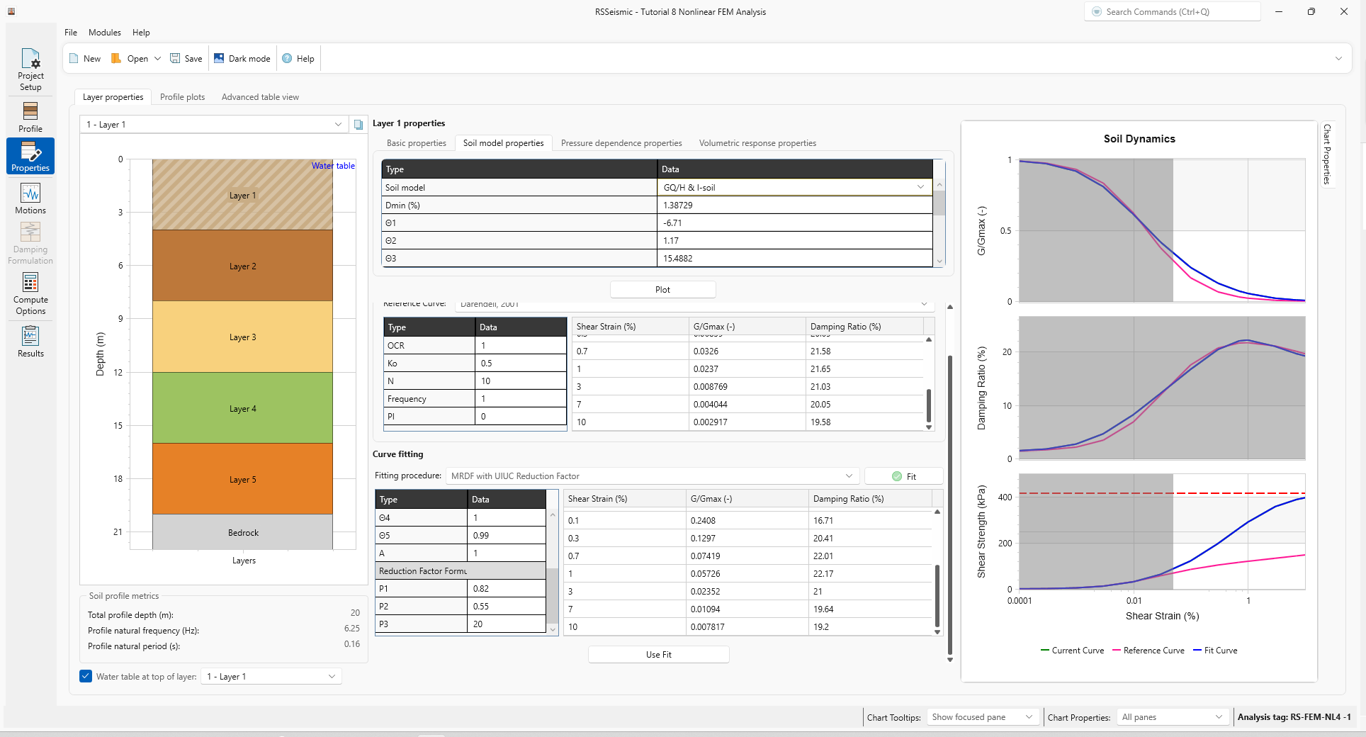
- Under Reference Curve > Sand select the Darendeli, 2001 reference curve.
- Enter Ko = 0.5. Leave all others values as the defaults shown below:
- OCR = 1
- Ko = 0.5
- N = 10
- Frequency = 1
- PI = 0
- Under Curve Fitting, enter Fitting Procedure = MRDF with UIUC Reduction Factor.
- Click Fit.
- The Fitting Limits dialog will appear. Leave the default values (Max strain = 0.05% and Min Strength = 95%) selected and click OK.
- The Soil model properties and Reduction factor formulation will be calculated. Click Use Fit to apply the fitted curve to Layer 1.
You can view the soil model properties by selecting the Soil model properties tab.
Select the Pressure dependence properties tab.
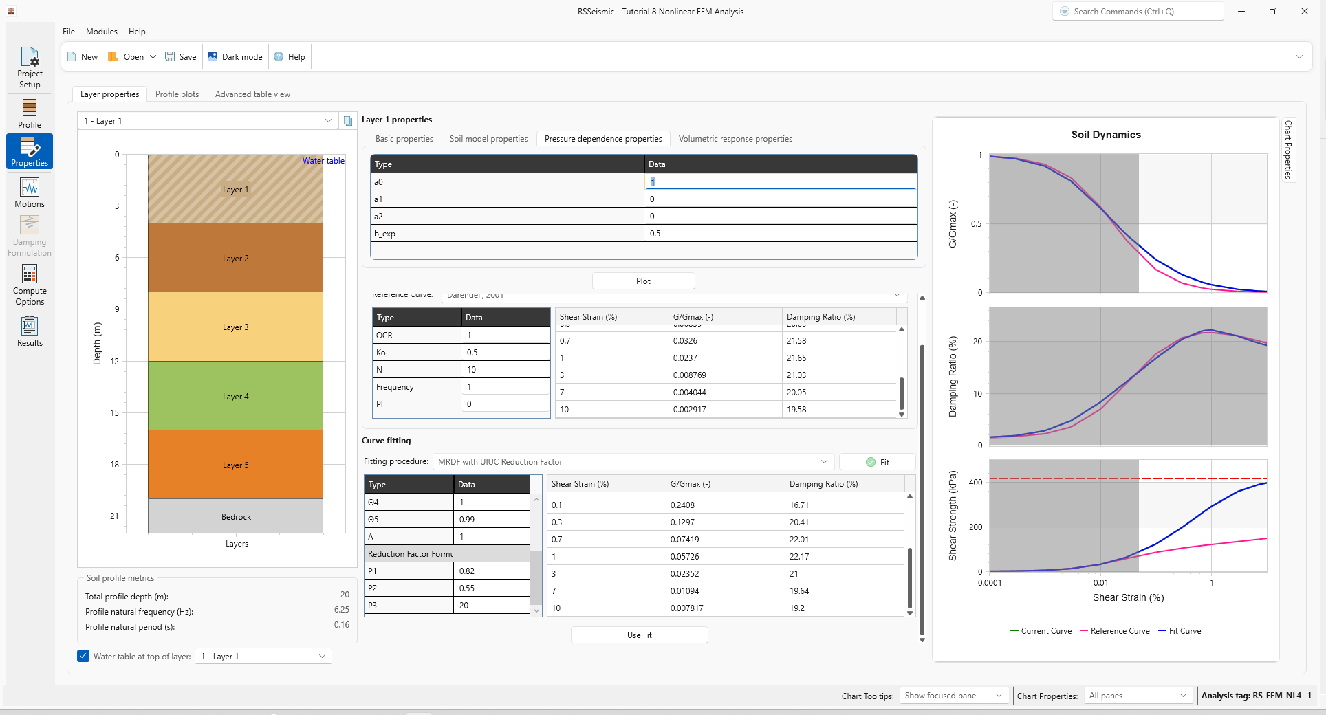
- We will leave the default values recommended by Numanoglu et al., 2023
Select the Volumetric response properties tab.
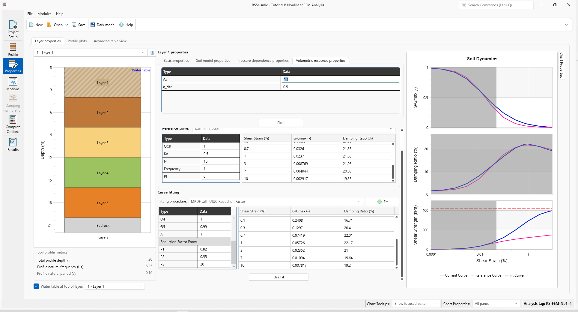
- We will leave the default values for this tab as well
- Repeat steps 3-10 above for layers 2-5. Use the basic properties listed in the table below to develop the fitted curves and use the corresponding model parameters.
| Name | Thickness (m) | Unit Weight (kN/ m3) | Shear Wave Velocity (m/s) | Shear Strength (kPa) | K0 | Poisson’s ratio (ν) |
| Layer 1 | 4 | 20 | 500 | 419.514 | 0.5 | 0.33 |
| Layer 2 | 4 | 20 | 500 | 443.046 | 0.5 | 0.33 |
| Layer 3 | 4 | 20 | 500 | 466.579 | 0.5 | 0.33 |
| Layer 4 | 4 | 20 | 500 | 490.112 | 0.5 | 0.33 |
| Layer 5 | 4 | 20 | 500 | 513.645 | 0.5 | 0.33 |
After completing the curve fitting for all the soil layers, select the Bedrock layer. Enter:
- Halfspace option = Elastic Halfspace
- Shear wave velocity (m/s) = 760
- Unit Weight (kN/m3) = 25
- Damping ratio (%) = 2
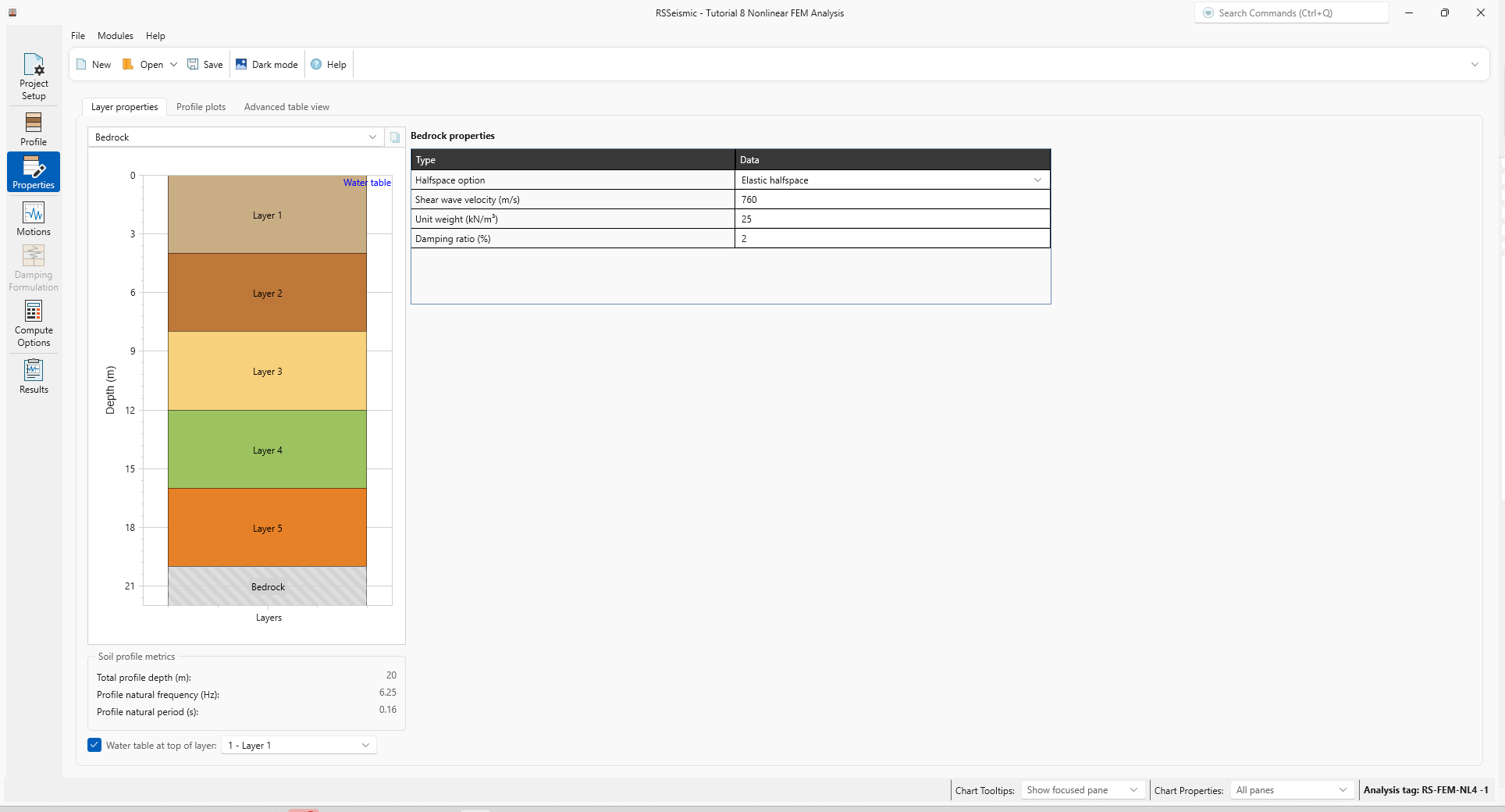
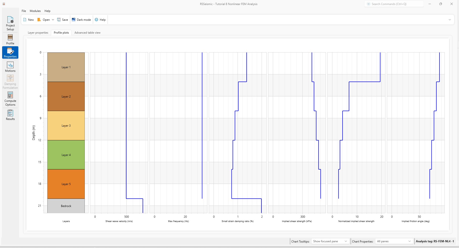
- Select the Profile Plots tab to review your data.
The user is encouraged to carefully examine these graphs to confirm that the input of selected profile characteristics are as intended. This includes shear wave velocity, the maximum frequency that can be propagated through the soil profile and implied strength properties.
5.0 Motions
- Select the Motions
 tab.
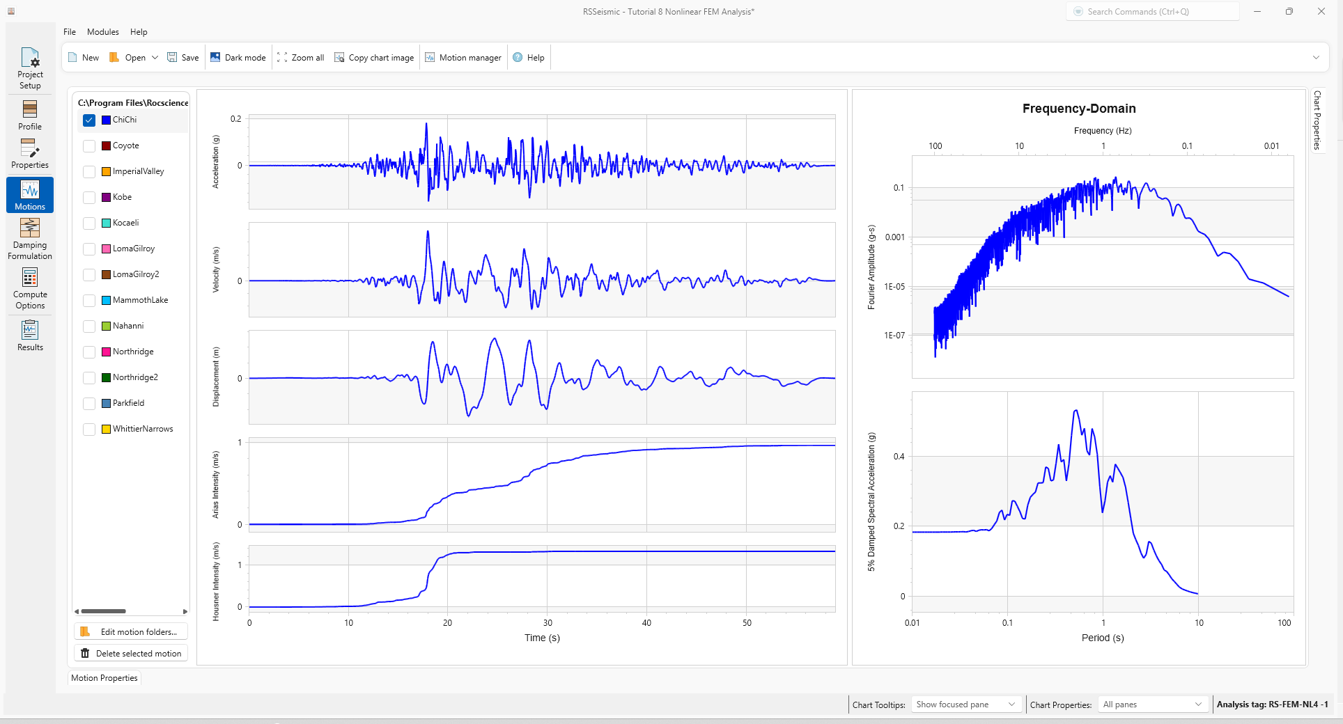
tab. - Under Resources\Input Motions, select ChiChi.
6.0 Damping Formulation
- Select the Damping Formulation
 tab.
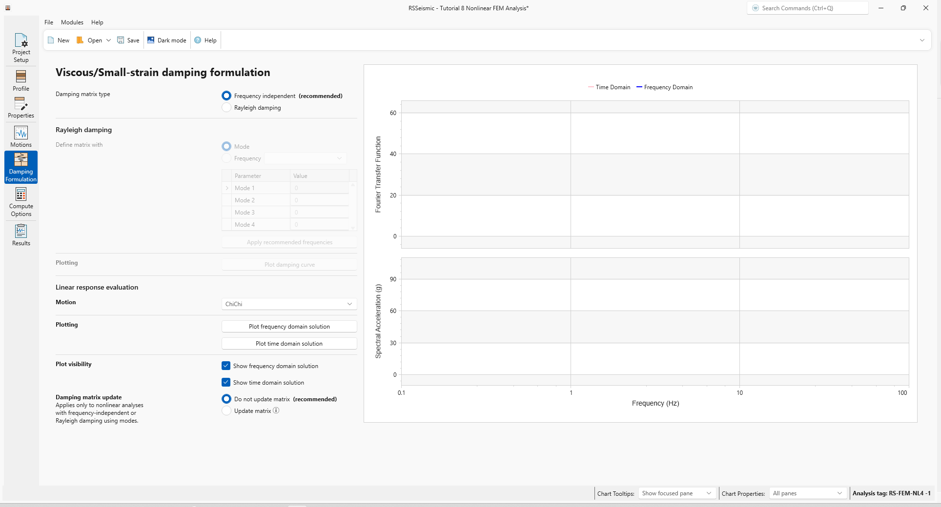
tab. - For Damping Matrix Type we will use the default selection of Frequency Independent.
7.0 Compute Options
Go to the Compute Options  tab.
tab.
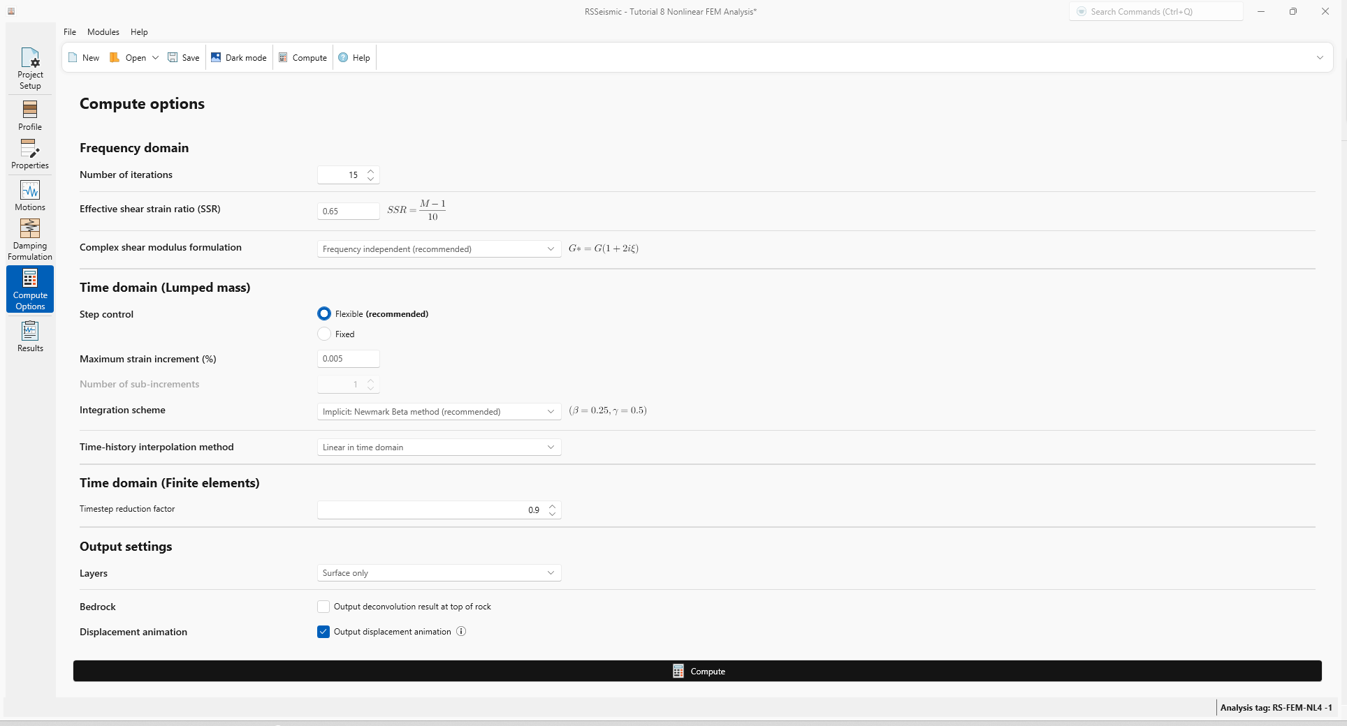
- For Frequency Domain use the default values:
- Number of iterations =15
- Effective Shear Strain Ratio (SSR) = 0.65
- Complex Shear Modulus Formulation = Frequency Independent
- For the Time Domain (Lumped mass) analysis use the default values:
- Step Control = Flexible
- Maximum Strain Increment (%) = 0.005 %
- Integration scheme = Implicit: Newmark Beta Method
- Time History Interpolation Method = Linear in time domain
- For the Time Domain (Finite Elements) analysis use the default values:
- Timestep reduction factor = 0.9
- For Output settings ensure Layers = Surface only is selected.
- Click Compute
8.0 Results
- Go to the Results
 tab.
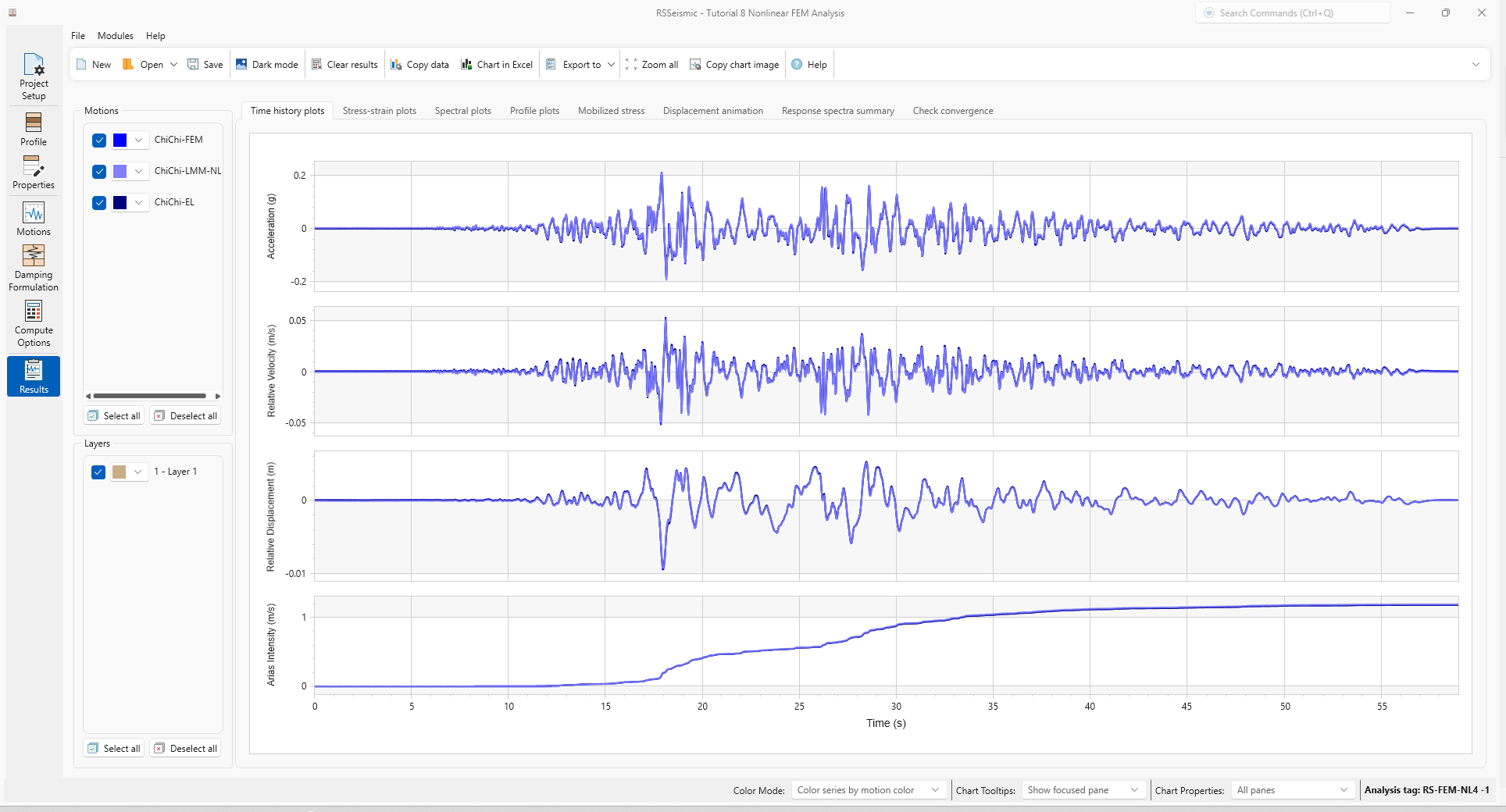
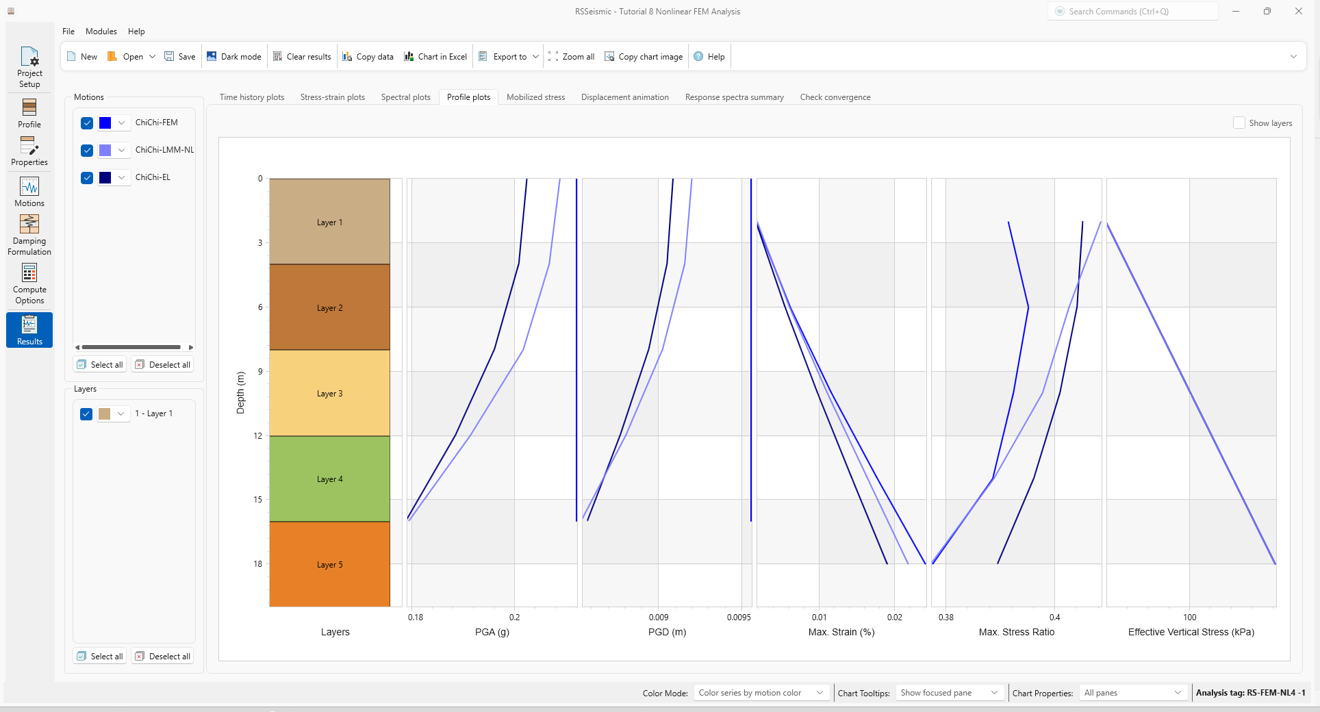
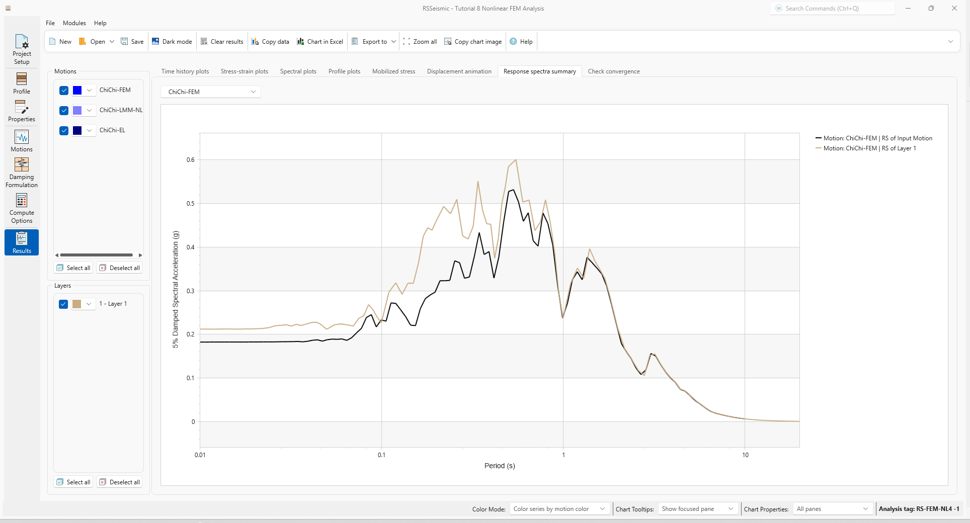
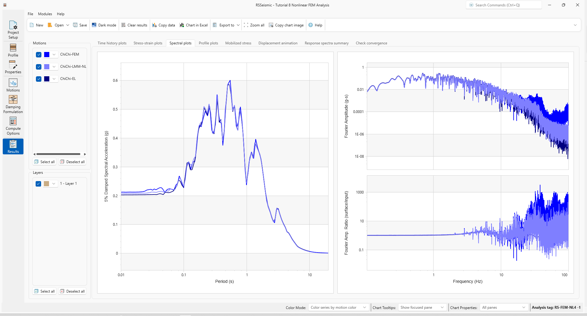
tab. - The Time History, Profile, Response Spectra Summary, and Spectral Plots should look as follows: