6 - Joint Persistence Analysis

In this tutorial, we look at the Probabilistic analysis of a slope, taking into account the persistence distribution of the joints and the spatial variation of the location of the joints. We then compare these results with the results of a standard SWedge analysis that uses maximum wedge size.

Topics Covered in this Tutorial:

• Persistence Analysis
• Limiting Wedge Size
• Slope Length
• Bench Width
• Persistence Distribution
• Exponential Distribution
• Wedge Spatial Location

Finished Product:

The finished product of this tutorial can be found in the Tutorial 06 Persistence Analysis.swd7 file, located in the Examples > Tutorials folder in your SWedge installation folder.

1.0 Introduction

In standard SWedge analysis, the program always tries to determine the maximum size wedge (i.e., it automatically scales a wedge to fit the dimensions of the slope). Joint Persistence, joint Trace Length, wedge Volume, and wedge Weight can also be used to scale the wedge size. In all cases, the program generates a wedge if possible.

In a Probabilistic analysis, this has a conservative effect on the Probability of Failure. In many cases, the spatial location and persistence of the joints limit the existence of valid wedges. In the case of a slope with a particular Length, Height, and Bench Width, only certain spatial locations of the joint planes result in valid wedges. In the case of Persistence, a wedge does not form if the joint Persistence is below a certain value.

SWedge has the ability to take these factors into consideration in a Probabilistic analysis. Using the Persistence Analysis option, you can both spatially vary the location of the joint planes and define statistical distributions of either Persistence or Trace Length. Using this option, you can refine your calculation of the Probability of Failure.

2.0 Creating a New File

1. If you have not already done so, run the SWedge program by double-clicking the SWedge icon in your installation folder or by selecting Programs > Rocscience > SWedge > SWedge in the Windows Start menu.

When the program starts, a default model is automatically created. If you do NOT see a model on your screen:

2. Select: File > New

Whenever a new file is created, the default input data forms valid slope geometry, as shown in the image below.

If the SWedge application window is not already maximized, maximize it now so that the full screen is available for viewing the model.

Notice the four-pane, split-screen format of the display, which shows Top, Front, Side and Perspective views of the model. This view is referred to as the Wedge View. The Top, Front and Side views are orthogonal with respect to each other (i.e., viewing angles differ by 90 degrees.)

3.0 Model

3.1 PROJECT SETTINGS

Let's start by setting up the project in the Project Settings dialog.

1. Select: Analysis > Project Settings
2. Select the General tab.
3. Change the Analysis Type to Probabilistic.
4. Set Units = Metric, stress as MPa.
5. Select the Sampling tab.
6. Make sure Sampling Method = Latin Hypercube and Number of Samples = 10000.
7. Select the Random Numbers tab.
8. Make sure Random Number Generation method = Pseudo-random and that the Specify Seed check box is UNCHECKED.
9. Click OK.

3.2 INPUT DATA

Now let’s define the slope and joint properties in the Input Data dialog.

1. Select: Analysis > Input Data
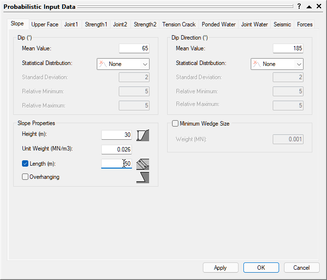
2. Select the Slope tab.
3. Set Dip Mean Value = 65, Dip Direction Mean Value = 185, and Slope Properties Height = 30.
4. Make sure Statistical Distribution for both Dip and Dip Direction are set to None.
5. Make sure Slope Properties Unit Weight (MN/m3) = 0.026.
6. Select the Slope Properties Length (m) check box and enter 50.



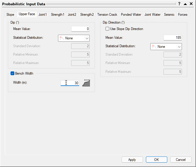
7. Select the Upper Face tab.
8. Set Dip Mean Value = 0, Dip Direction Mean Value =185.
9. Make sure Statistical Distribution for both Dip and Dip Direction are set to None.
10. Select the Bench Width option and set Width (m) = 30.



11. Select the Joint1 tab.
12. Change the Orientation Definition Method to Fisher Distribution.
13. Set Mean Dip Value = 45 and Mean Dip Direction Value =125.
14. Enter a Standard Deviation of 10.
15. Keep Waviness Mean Value = 0 and Statistical Distribution = None.



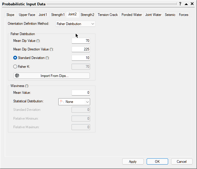
16. Select the Joint 2 tab.
17. Change the Orientation Definition Method to Fisher Distribution.
18. Set Mean Dip Value = 70 and Mean Dip Direction Value = 225.
19. Enter a Standard Deviation of 10.
20. Keep Waviness Mean Value = 0 and Statistical Distribution = None.



21. Select the Strength1 tab.
22. Change the Strength Model to Barton-Bandis and make sure Random Variables = Parameters.
23. Set JRC Mean Value = 6, JCS Mean Value = 50, and Phir Mean Value = 25.
24. Make sure all Statistical Distribution = None.



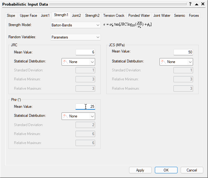
25. Select the Strength 2 tab and enter the same parameters as Strength 1
26. Click the OK button to save your changes, compute the probability of failure, and close the Input Data dialog.

4.0 Analysis Results

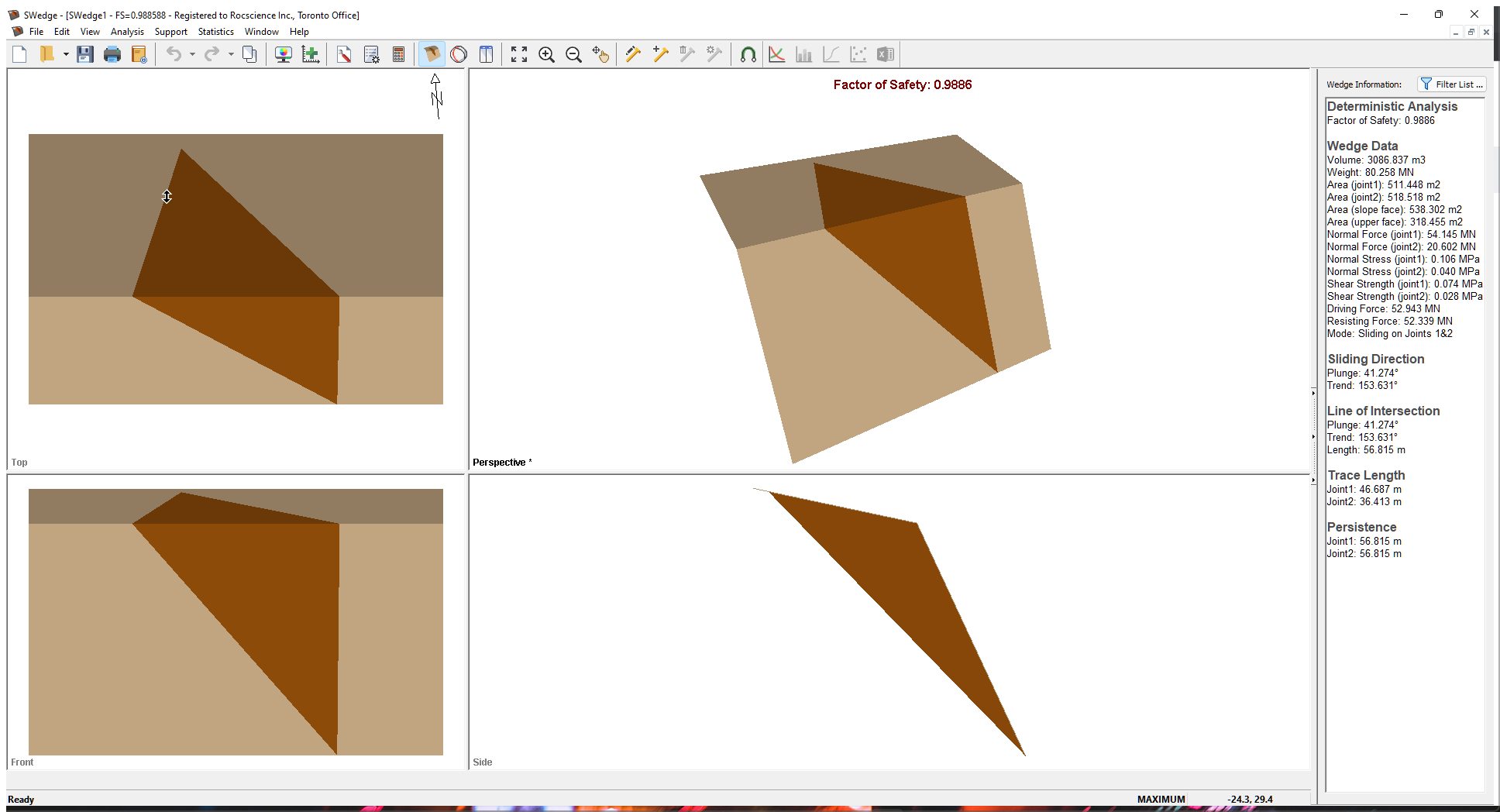
Computation of 10000 Latin Hypercube samples occurs and the Probability of Failure is calculated, as shown in the figure below.

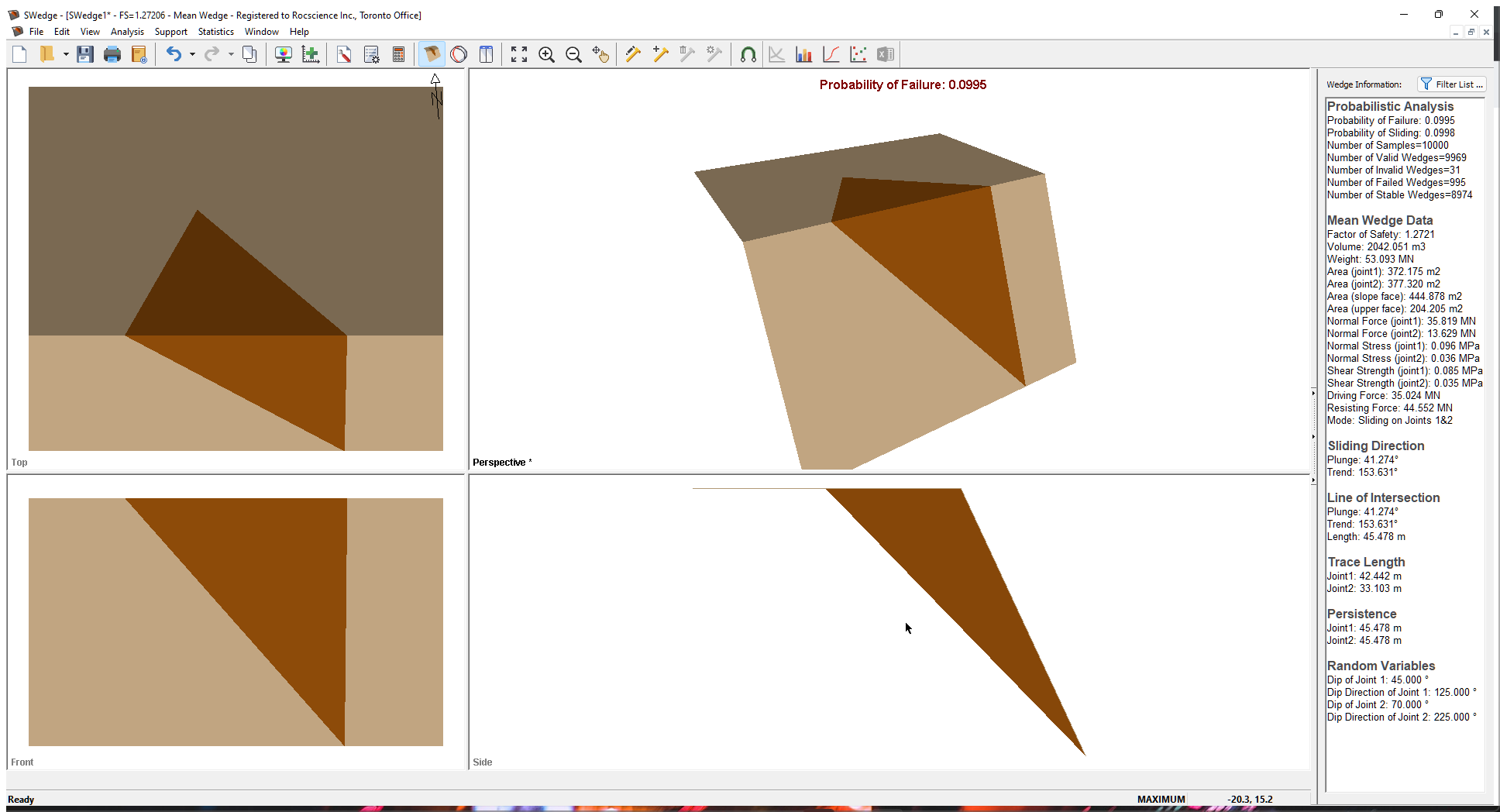
Note the following:

• The only Random Variables are the orientation of the joints.
• The results of the Probabilistic analysis are summarized in the Wedge Information Panel in the application Sidebar. The wedge computed using the mean values of all the input parameters is displayed with its Factor of Safety results.
• The Probability of Failure is 0.0995 or 9.95%. Out of the 10000 samples, 9969 produced Valid Wedges. Of these 9969, 995 had a Factor of Safety of less than 1.0 (failed), calculated as #failed/total #samples = Probability of Failure =995/10000=0.0995.
• The Mean Wedge has a Factor of Safety of 1.27
• It's important to remember that SWedge does its best to fit a wedge inside the slope dimensions, i.e., tries to determine a maximum size wedge for any slope geometry. It adjusts the location of the joints in order to determine this maximum size wedge.
• The Probability of Failure is conservative (upper bound solution) since positional information and joint length are not accounted for and the maximum size wedge is computed.

5.0 Persistence Analysis

As just noted, both the joint length and the positional location of the joints are not accounted for by default. This results in a conservative upper bound solution for the Probability of Failure. To refine the computation, SWedge allows you to define statistics for both the joint location and joint length (in terms of either Persistence or Trace Length).

In addition, two different Joint Spacing options are available for a Persistence analysis:

1. Large Joint Spacing
2. Small Joint Spacing (Ubiquitous Joints)

5.1 LARGE JOINT SPACING

With the Large Joint Spacing option, it is assumed there is only one trace of Joint 1 and one trace of Joint 2 on the slope face. The point of intersection of the two joint planes on the slope face is randomly located somewhere between the toe and crest of the slope, resulting in a uniform distribution of wedge height (measured vertically from this intersection point to the slope crest).

Once the intersection point has been selected, orientations for each joint are determined. If a valid wedge forms, the required joint length (JR) is calculated for each joint and compared to the deterministic or sampled joint length from user inputs (JS). If the required length exceeds the sampled length, the wedge is considered “invalid”. Otherwise, the wedge is valid and the Factor of Safety is calculated.

Note that, if the spatial location of the joints is not uniformly random, the wedge height should NOT be uniformly varied, as this could lead to an under-/ over-estimation of the Probability of Failure.

The Large Joint Spacing option is a lower bound solution when it comes to Probability of Failure, as the spacing and persistence condition limits the formation of wedges.

5.2 SMALL JOINT SPACING

Now consider the case where there is spacing (repeated joints) associated with the two joint sets Joint 1 and Joint 2. There is no longer one wedge but a number of possible wedges that can form on the slope. If a wedge cannot form because the Persistence is not large enough, a wedge that meets the Persistence conditions can form higher up the slope face. If this is the case, the Small or Ubiquitous Joint Spacing option is more applicable. This option automatically scales down the wedge size until the Persistence conditions are met. Therefore, a wedge is almost always formed in each simulation if the geometry of the joints and slope creates a kinematically feasible wedge. Its size is dependent on the sampled Persistence and the geometry of the bench.

The Small Joint Spacing option is an upper bound solution for Probability of Failure because the program always creates a wedge independently of any spatial location of the joints on the slope face. The only thing that limits the size of the wedge is the geometry of the bench and the Persistence of the joints.

5.3 PERSISTENCE ANALYSIS

We'll now perform a Persistence analysis using the Large Joint Spacing option.

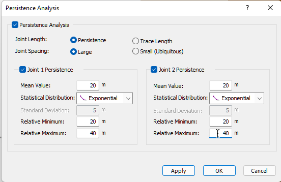
1. Select Analysis > Persistence Analysis to open the Persistence Analysis dialog.
2. Select the Persistence Analysis check box.
3. Make sure the Persistence option is selected for Joint Length.
4. Make sure Large is selected for the Joint Spacing option.
   By selecting this option, the location of the joint planes varies uniformly throughout the slope face. The point of intersection of the two joint planes on the slope face is randomly located somewhere between the toe and crest of the slope. The height of the wedge, measured vertically from this intersection point to the slope crest, is a uniform distribution varying between zero and the slope height.
5. Select both the Joint 1 Persistence and Joint 2 Persistence checkboxes and set the Statistical Distribution for both to Exponential.
6. For both Joint 1 Persistence and Joint 2 Persistence, enter a Mean Value of 20, a Relative Minimum of 20, and a Relative Maximum of 40.
   This results in the Joint Persistence varying exponentially between 0 and 50 m with a mean of 20 m.
7. Click OK to save your changes, compute the Probability of Failure, and close the Persistence Analysis dialog.

6.0 Persistence Analysis Results

Computation of 10000 Latin Hypercube samples occurs and the Probability of Failure is calculated. For every one of the 10000 simulations, a value of Joint Persistence is sampled. Because the Large Joint Spacing option is selected, if the wedge that is formed based on the random location of the joint planes has Joint Persistence values that exceed the sampled values, the wedge is flagged as invalid.

The figure below illustrates the results of this computation.

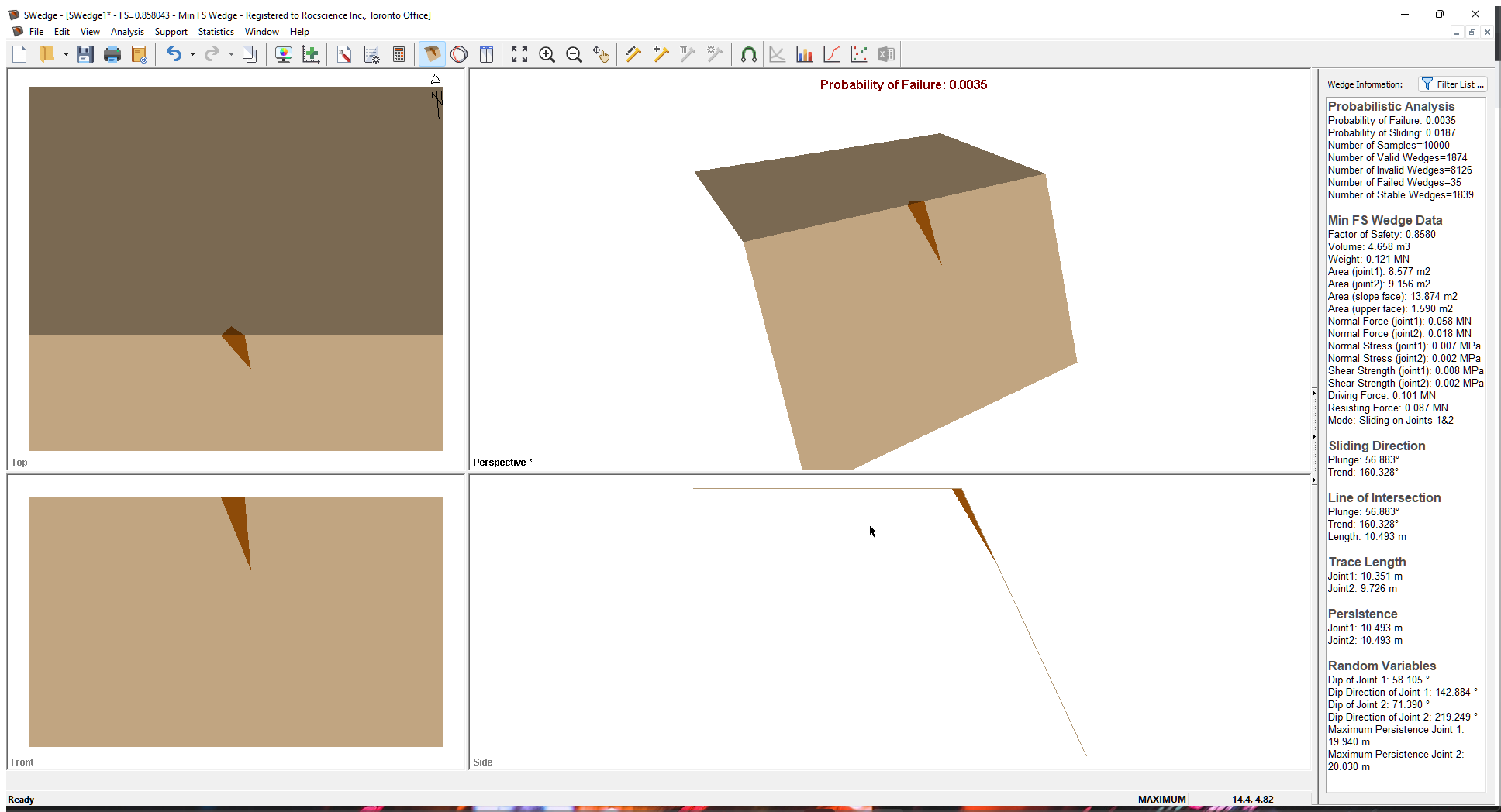
Note the following:

• The random variables now include the height of the wedge and the Maximum Persistence of the joints.
• The Probability of Failure is reduced from 0.0995 to 0.0035 (28 times smaller).
• The Number of Valid Wedges has been reduced from 9969 to 1874. This is because the program no longer tries to fit a wedge inside the slope dimensions by adjusting the location of the joints. If the location and length of the joint planes are not sufficient to produce a valid wedge, the wedge is flagged as invalid.
• The Number of Failed Wedges is reduced from 995 to 35 for the same reasons.
• In general, the Probability of Failure from a Persistence analysis is more accurate because it accounts for the spatial location and length of the joint planes.

7.0 Histogram Plots of Results

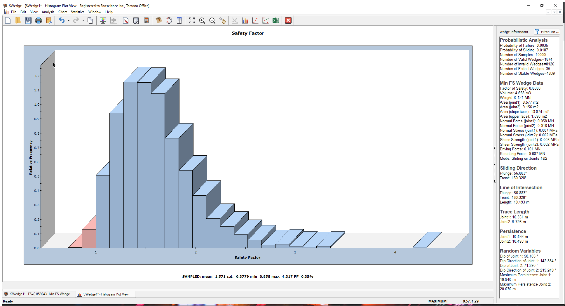
A number of useful features exist for the display of data from a Probabilistic analysis. For example, to get an idea of the relative distribution of failed to stable samples, we can plot a histogram of the Factor of Safety. To open the Histogram Plot Parameters dialog:

1. Select: Statistics > Plot Histogram
2. Leave the Data Type as Safety Factor.
3. Click the OK button.
   A Safety Factor histogram is displayed.
4. Right-click in the histogram and select 3D Histogram from the popup window.

Now let’s plot the maximum Persistence of Joint 1 that was statistically generated as part of the Persistence analysis.

5. Re-open the Histogram Plot Parameters dialog.
6. In the Data Type drop-down, select Maximum Persistence Joint1 at the bottom of the list.
7. Select the Plot Input Distribution check box.
8. Click the OK button to generate the histogram.
9. Right-click in the plot and deselect Relative Frequency from the popup menu.
   This changes the y-axis of the histogram from Relative Frequency to the actual Frequency (i.e., the number of samples).
10. Right-click in the plot again and select Input Distribution from the popup menu.

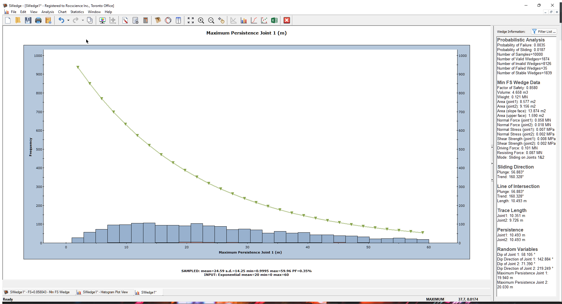
This is a plot of the sampled Maximum Persistence for Joint 1 for all VALID wedges. As mentioned above, for each one of the 10000 simulations, a Maximum Persistence value of the joint is sampled. If the wedge that is formed based on the random location of the joint planes has an actual Joint Persistence value that exceeds the sampled value, the wedge is flagged as invalid.

Remember that we defined an exponential distribution of Joint Persistence that varied between 0 m and 60 m with a mean of 20 m. Note that the histogram does not match this input distribution (the green line). This is because it does not include invalid wedges. Only the data from valid wedges is plotted by default.

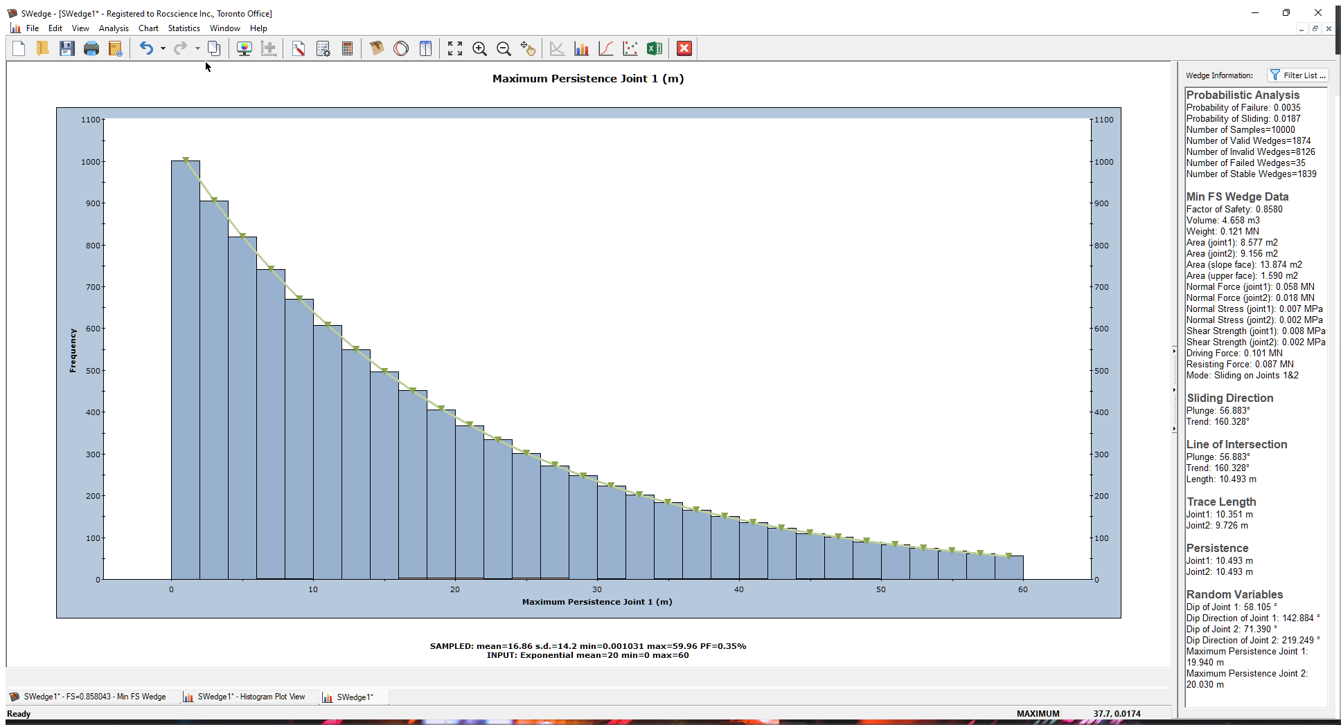
To see the distribution of all 10000 sampled Persistence values, right-click in the plot and select Include Invalid Wedges in the popup menu. The plot now includes all the sampled data (10000 samples), and the histogram bars match the input distribution.

Finally, let's look at a plot of the actual Persistence values for all the valid wedges.

1. Re-open the Histogram Plot Parameters dialog.
2. In the Data Type drop-down, select Persistence Joint 1.
3. Select the Best Fit Distribution check box.
4. Click OK.

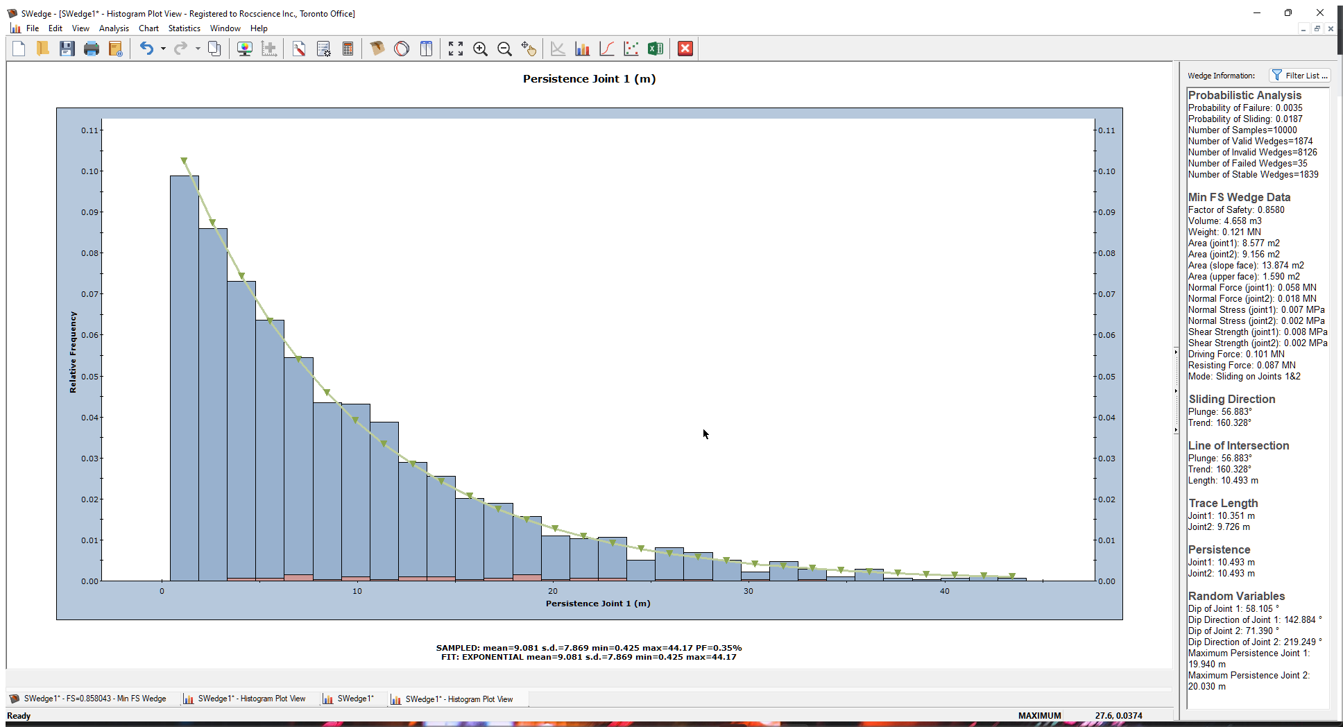
Note that most of the wedges have small Persistence values but a few have larger values. The Best Fit Distribution is also exponential. This is what one would expect for a joint set with exponentially varying Persistence.

This concludes the tutorial.