2 - Probabilistic Analysis

1.0 Introduction

In Tutorial 01 - Quick Start, you learned about the three main analysis types in SWedge: Deterministic, Probabilistic, and Combinations, and how to run a Deterministic analysis (the default). In this tutorial, you will learn how to run a Probabilistic analysis.

In a Probabilistic analysis, statistical input data can be entered to account for uncertainty in joint orientation and strength values. The result is a distribution of Factors of Safety, from which a Probability of Failure is calculated. To learn more about Probabilistic Analysis, see Overview of Probabilistic Analysis in SWedge.

Topics Covered in This Tutorial:

• Project Settings
• Random Variables
• Fisher Distribution
• Tension Crack
• Mean Wedge
• Picked Wedges
• Histograms
• Scatter Plots
• Stereonet View
• Show Failed Wedges
• Failure Mode Filter
• Design Factor of Safety

Finished Product:

The finished product of this tutorial can be found in the Tutorial 02 Probabilistic.swd7 file, located in the Examples > Tutorials folder in your SWedge installation folder.

2.0 Creating a New File

1. If you have not already done so, run the SWedge program by double-clicking the SWedge icon in your installation folder or by selecting Programs > Rocscience > SWedge > SWedge in the Windows Start menu.

When the program starts, a default model is automatically created. If you do NOT see a model on your screen:

2. Select: File > New

Whenever a new file is created, the default input data forms valid slope geometry, as shown in the image below.

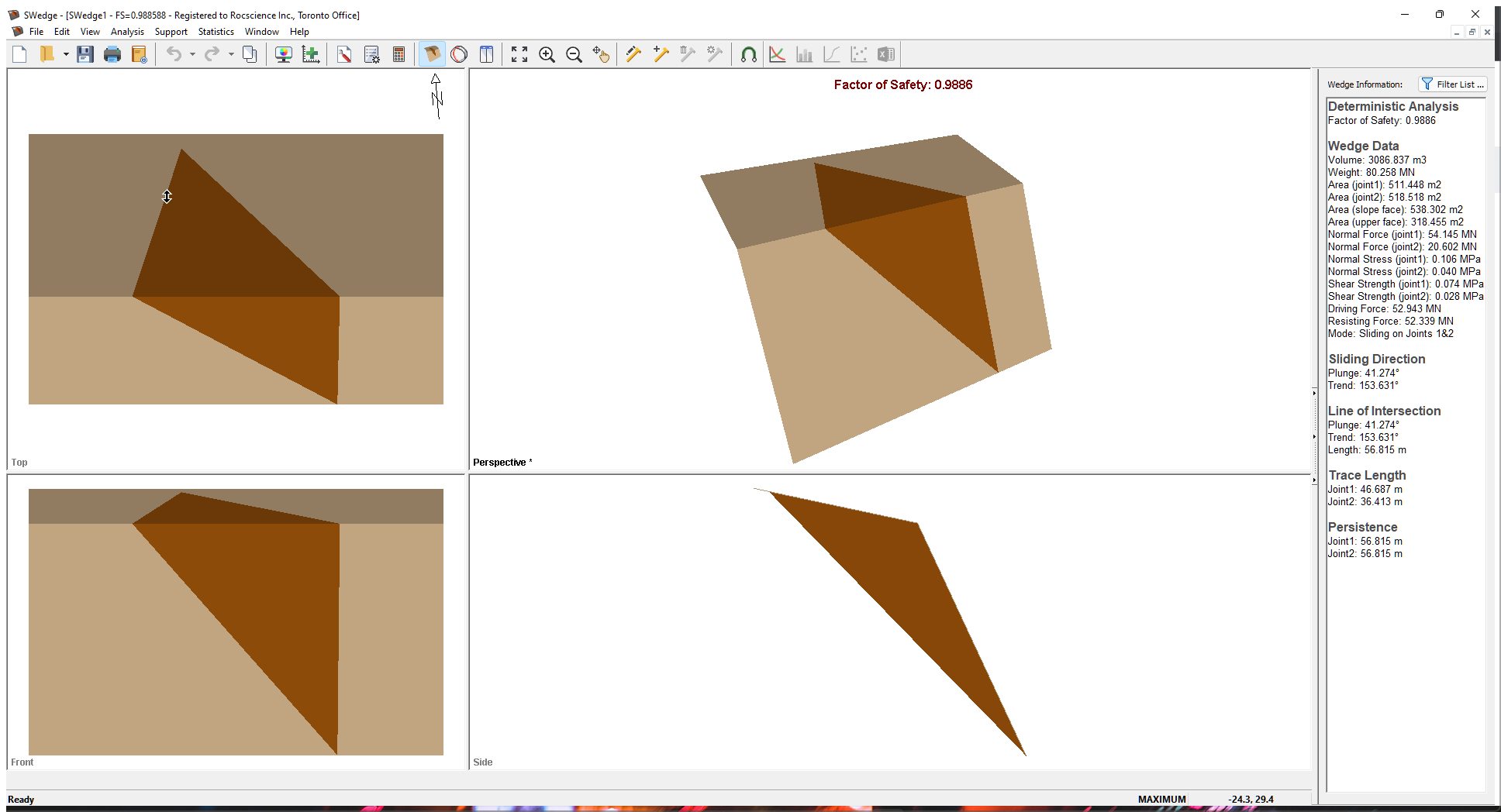
If the SWedge application window is not already maximized, maximize it now so that the full screen is available for viewing the model.

Notice the four-pane, split screen format of the display, which shows Top, Front, Side and Perspective views of the model. This view is referred to as the Wedge View. The Top, Front and Side views are orthogonal with respect to each other (i.e., viewing angles differ by 90 degrees.)

3.0 Project Settings

The Project Settings dialog allows you to configure the main analysis parameters for your model (i.e., Analysis Type, Units, Sampling Method, etc.).

1. Select: Analysis > Project Settings

3.1 ANALYSIS TYPE AND BLOCK SHAPE

By default a Deterministic analysis is selected for a new file.

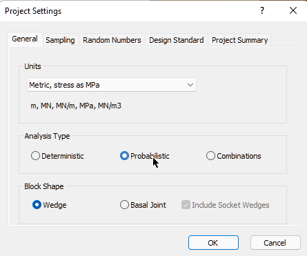
1. Select the General tab.
2. Change the Analysis Type to Probabilistic.
3. Keep Block Shape as Wedge.

3.2 UNITS

For this tutorial we will be using Metric units, so make sure the Metric, stress as MPa option is selected for Units.

3.3 SAMPLING AND RANDOM NUMBERS

1. Select the Sampling tab.



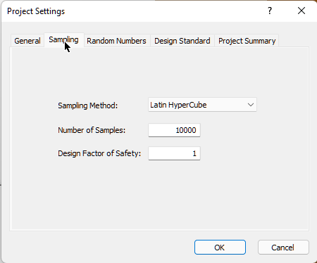
The Sampling Method determines how the statistical distribution for the random input variables will be sampled. The default settings are Sampling Method = Latin Hypercube and Number of Samples = 10,000. For more help, see Sampling in SWedge Project Settings.

Note the Design Factor of Safety option. This option is used in Probabilistic and Combinations analyses to determine both the Probability of Failure and the number of failed wedges in graphs. The Probability of Failure is now P(FS < Design FS). For this tutorial, keep Design Factor of Safety = 1.

2. Select the Random Numbers tab.

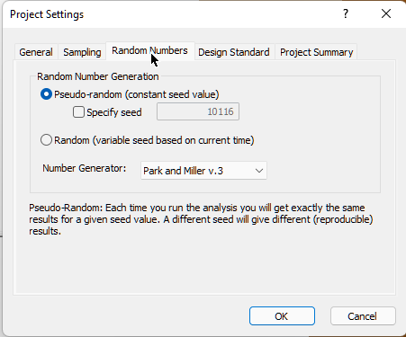
Note that Random Number Generation is set to Pseudo-random by default. This allows you to obtain reproducible results for a Probabilistic analysis by using the same seed value to generate random numbers. We will discuss Pseudo-random versus Random sampling later in this tutorial.

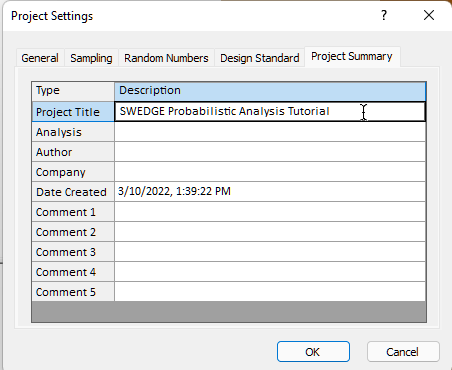
3.4 PROJECT SUMMARY

1. Select the Project Summary tab and enter "SWedge Probabilistic Analysis Tutorial" as the Project Title.



NOTE: You can have Project Summary information appear on analysis results printouts by setting up a header or footer through Page Setup on the File menu.
2. Click OK to close the Project Settings dialog.

4.0 Probabilistic Input Data

To enter input data for the Probabilistic analysis:

1. Select: Analysis > Input Data

For a Probabilistic analysis, the Input Data dialog is organized under several tabs as shown below.

To carry out a Probabilistic analysis with SWedge, at least one input parameter must be defined as a random variable. To define a random variable, you select a statistical distribution (e.g., Normal, Lognormal, Fisher, etc.) for the variable and enter appropriate parameters (e.g., Standard Deviation, Relative Minimum, Relative Maximum, etc.).

For the example in this tutorial, we will define the following input parameters as random variables:

• Joint 1 orientation
• Joint 1 shear strength
• Joint 2 orientation
• Joint 2 shear strength
• Tension Crack orientation

All other input parameters are assumed to be exactly known (i.e., Statistical Distribution = None) and will not be involved in the statistical sampling.

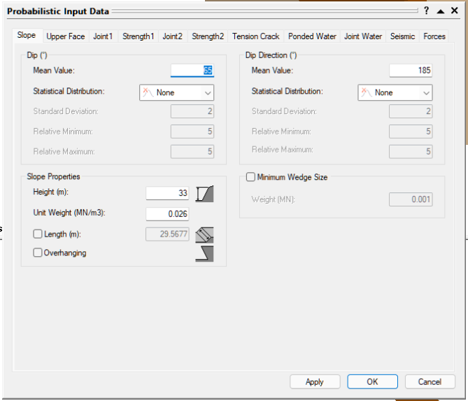
4.1 SLOPE

1. Select the Slope tab.

For this tutorial, we assume the orientation of the slope plane is constant so we won't set any statistical distributions in this tab.

2. Keep all Statistical Distribution parameters set to None.
3. Keep the default orientation Mean Values as Dip = 65, Dip Direction = 185.
4. Set Slope Properties Unit Weight MN/m³ = 0.026 .
5. Set Slope Properties Height (m) = 20.
6. Select the Slope Properties Length (m) check box and enter 60.

4.2 UPPER FACE

1. Select the Upper Face tab.

For this tutorial, we assume the orientation of the upper face is constant so we won't set any statistical distributions in this tab.

2. Keep all Statistical Distribution parameters set to None.
3. Keep the default orientation Mean Values as Dip = 12, Dip Direction = 185).
4. Select the Bench Width check box and set Width (m) = 15.

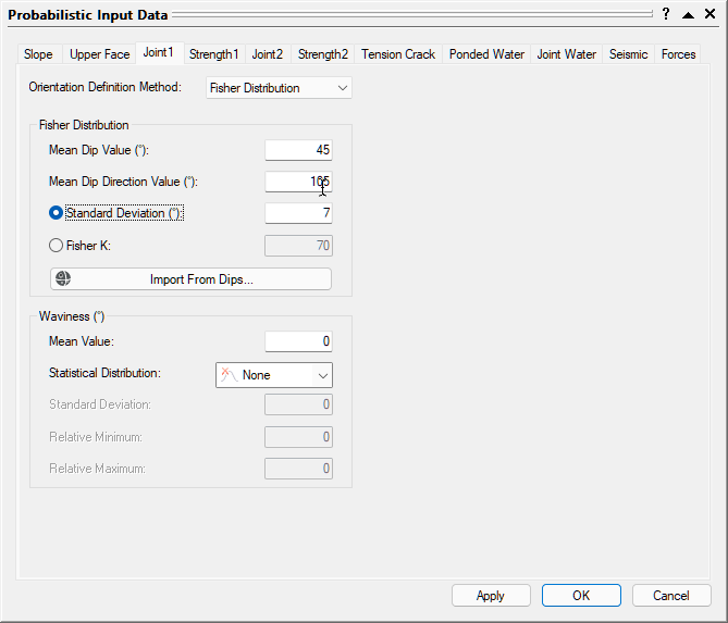
4.3 JOINT 1 ORIENTATION

1. Select the Joint 1 tab.

Note that there are two methods of defining the variability of joint orientation (Orientation Definition Method):

• Dip/Dip Direction: The Dip and Dip Direction are treated as independent random variables (i.e., you can define different statistical distributions for each one).
• Fisher Distribution: Generates a symmetric, three-dimensional distribution of orientations around the mean plane orientation, so only a single standard deviation is required. In general, a Fisher Distribution is recommended for generating random joint plane orientations because it provides more predictable orientation distributions and lessens the chance of input data errors.

For this tutorial, we are using the Fisher Distribution option.

2. Set Orientation Definition Method = Fisher Distribution.
3. Set Mean Dip Value = 45, Mean Dip Direction Value = 105, and Standard Deviation = 7.

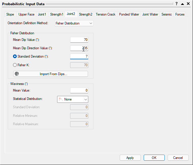
4.4 JOINT 2 ORIENTATION

1. Select the Joint 2 tab.
2. Set Orientation Definition Method = Fisher Distribution.
3. Set Mean Dip Value = 70, Mean Dip Direction Value = 235, and Standard Deviation = 7.

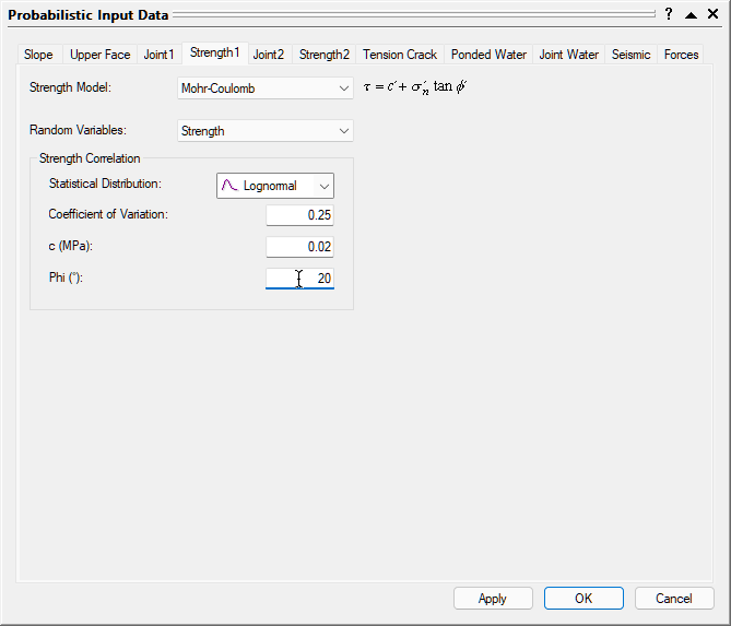
4.5 JOINT 1 STRENGTH

1. Select the Strength 1 tab.

Note that there are two methods of defining the statistical variability of joint shear strength (Random Variables):

• Parameters: The individual strength criterion parameters (e.g., cohesion and friction angle) can each be assigned a statistical distribution.
• Strength: The shear strength variability is defined with respect to the mean strength envelope. This method has the advantage of requiring only a single parameter (coefficient of variation) to define the shear strength variability.

2. Set Random Variables = Strength.
3. Set Statistical Distribution = Lognormal.
4. Set Coefficient of Variation = 0.25, Cohesion (c [MPa]) = 0.02, and Phi [deg] = 20.

NOTES:

• The Coefficient of Variation is defined as the Standard Deviation (of the shear strength) divided by the Mean (shear strength).
• Only Lognormal and Gamma distributions are allowed when defining shear strength as a random variable because they are defined only for positive values. This ensures that the randomly generated values of shear strength are always positive (negative shear strength has no physical meaning in SWedge).

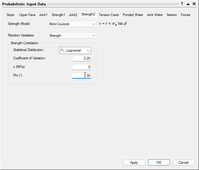
4.6 JOINT 2 STRENGTH

1. Select the Strength 2 tab.
2. Set Random Variables = Strength.
3. Set Statistical Distribution = Lognormal.
4. Set Coefficient of Variation = 0.25, Cohesion (c [MPa]) = 0, Phi [deg] = 30.

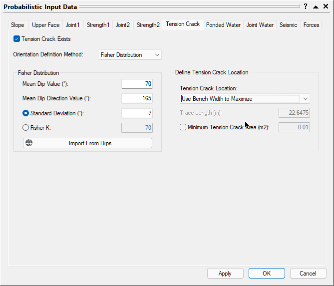
4.7 TENSION CRACK

1. Select the Tension Crack tab.

For this tutorial, we'll include a tension crack in the model and define the orientation as a random variable.

2. Select the Tension Crack Exists check box.
3. Set Orientation Definition Method = Fisher Distribution.
4. Set Mean Dip Value = 70, Mean Dip Direction Value = 165, and Standard Deviation = 7.
5. For Define Tension Crack Location, set Tension Crack Location = Use Bench Width to Maximize from the dropdown.

5.0 Compute

1. Click OK in the Input Data dialog to compute the SWedge Probabilistic analysis.

SWedge uses the Latin Hypercube sampling method to generate 10,000 random input data samples for each random variable, using the specified Statistical Distributions, and to compute the Factor Safety for 10,000 possible wedges. The calculation takes only a few seconds, and the progress of the calculation is indicated in the status bar.

TIP: You can also click the Apply button in the Input Data dialog to compute the analysis without closing the dialog. This allows you to easily test different input parameters and re-compute the results.

6.0 Probabilistic Analysis Results

This is the first result reported in the Probabilistic Analysis section of the Wedge Information Panel in the application Sidebar.

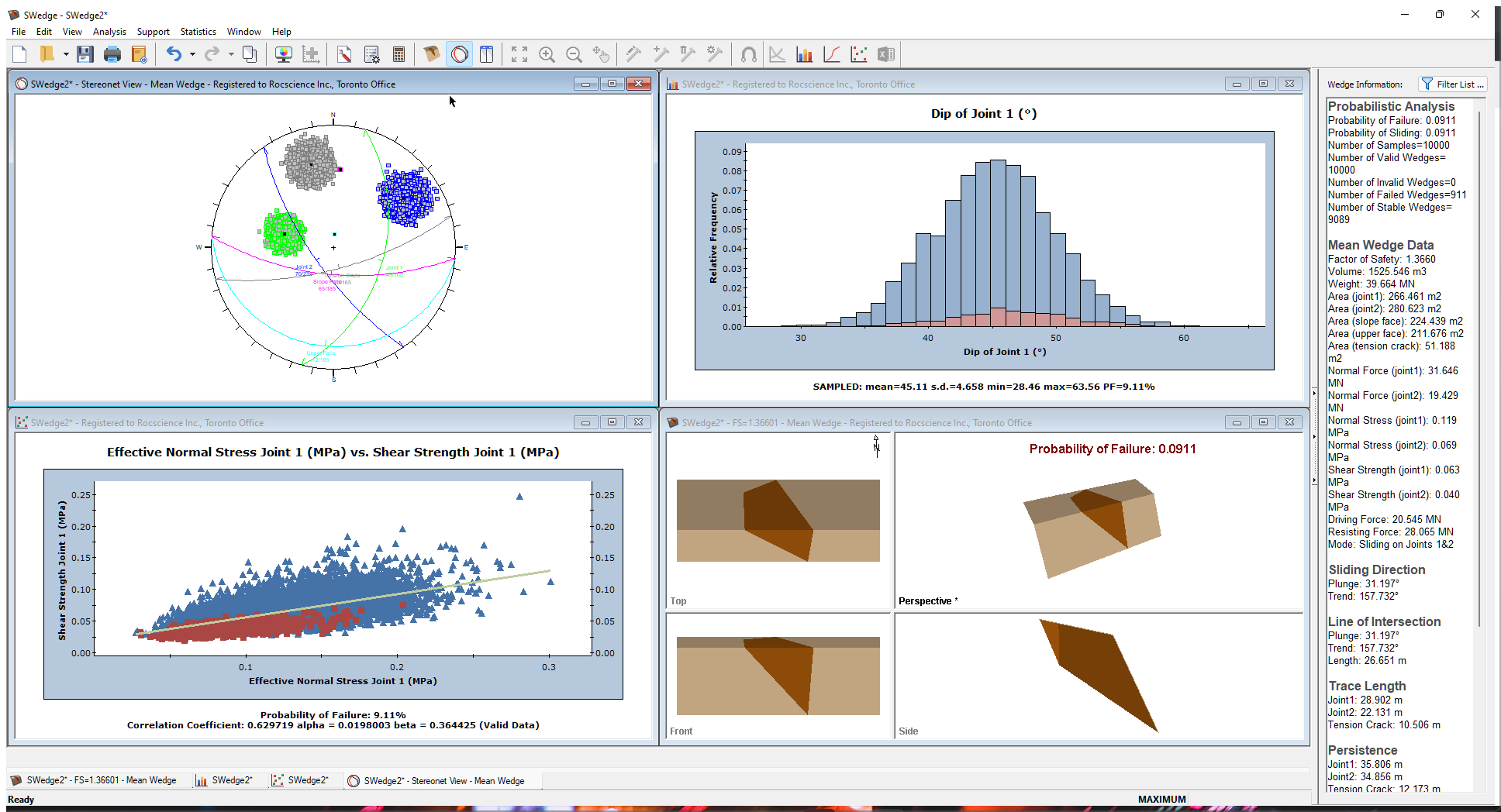
For this example, if you entered the Input Data correctly, you should obtain a Probability of Failure (PF) of about 9% (PF = 0.0911).

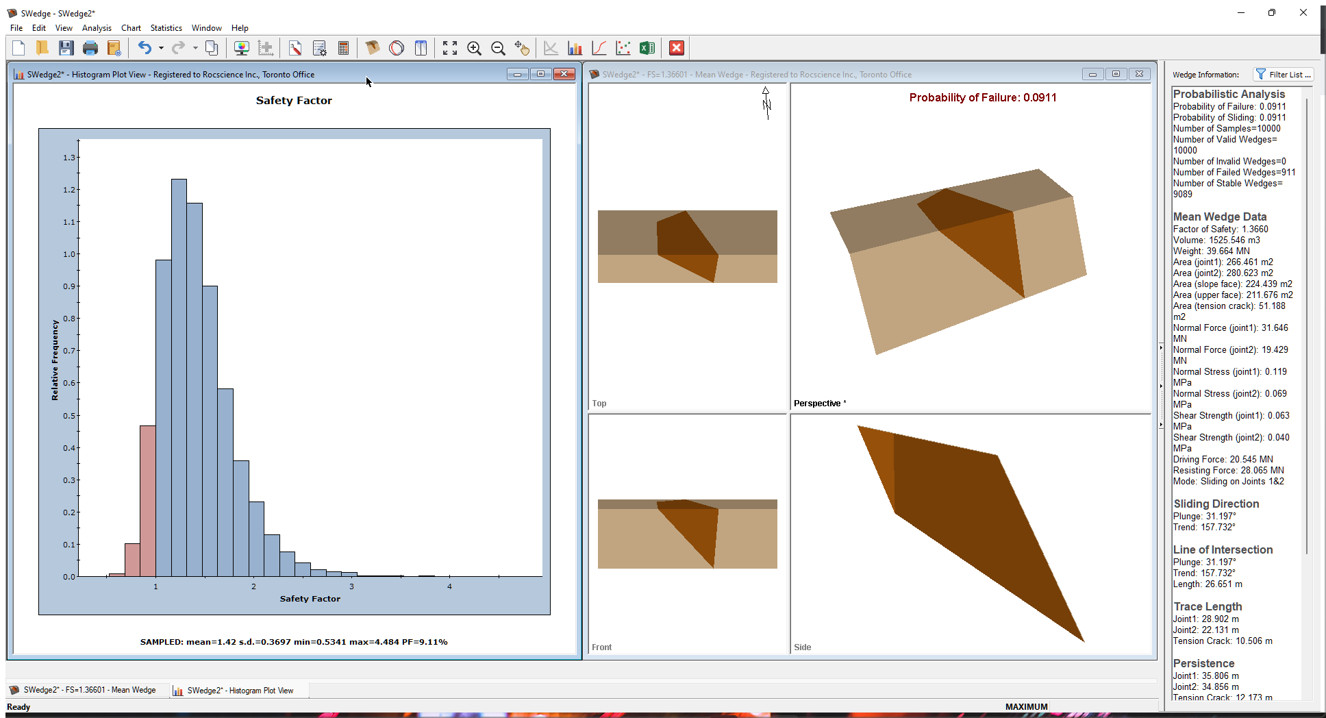
6.1 WEDGE INFORMATION PANEL

A summary of analysis results is displayed in the Wedge Information Panel in the application Sidebar.

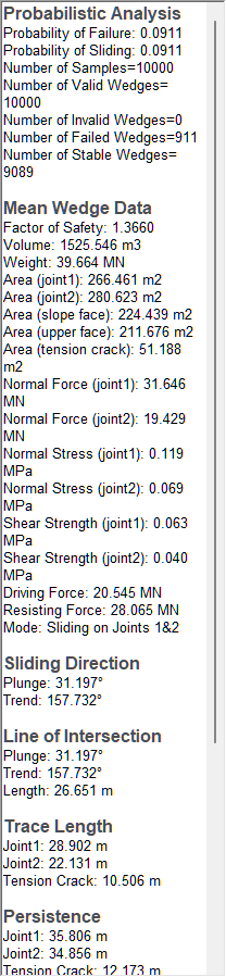
The primary result of interest from a Probabilistic analysis is the Probability of Failure, which is the first result shown in the Probabilistic Analysis section of the panel. If you entered the input data correctly, you should obtain a Probability of Failure of about 9% (0.0911).

Note that the Probability of Failure is equal to the Number of Failed Wedges (i.e., those with a Factor of Safety < 1) divided by the Number of Samples (as entered in the Project Settings dialog), i.e., 911 / 10000.

6.2 WEDGE VIEW

The wedge displayed by default in the Wedge View after a Probabilistic analysis is based on the Mean Values entered in the Probabilistic Input Data dialog and is referred to as the Mean Wedge. The Factor of Safety of the Mean Wedge should be 1.3660, as shown in the Wedge Information Panel.

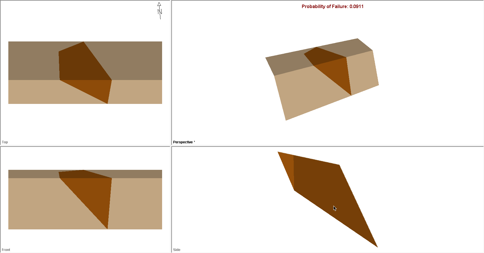
Note that the Tension Crack for the Mean Wedge is positioned to create the maximum wedge size for the given bench width (remember that the Use Bench Width to Maximize option is in effect).

To view the wedge with the minimum Factor of Safety generated by the Probabilistic analysis, right-click in the Wedge View and select Show Min FS Wedge from the popup menu. The analysis information now shown in the Wedge Information Pane is now for the wedge with the minimum Factor of Safety (should be 0.534).

To restore the Mean Wedge display and information, right-click in the Wedge View and select Show Mean FS Wedge.

6.3 HISTOGRAM VIEW

To plot histograms of results after a Probabilistic analysis:

1. Select: Statistics > Plot Histogram
   
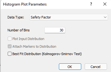
2. Click OK to plot a Safety Factor histogram.

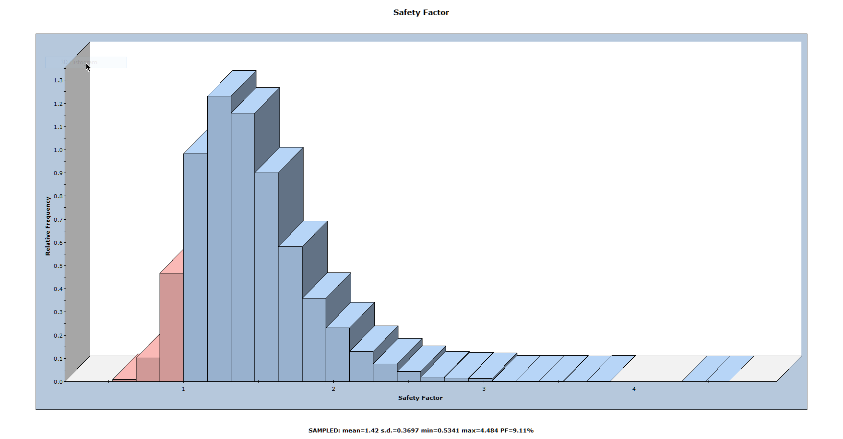
The histogram displayed in the Histogram View represents the distribution of the Factor of Safety for all valid wedges generated by the random sampling based on data entered in the Input Data dialog. The red bars on the left of the distribution represent wedges with a Factor of Safety of less than 1.0.

To display the histogram bars in 3D, right-click in the histogram and select 3D Histogram from the popup menu

6.3.1 Mean Factor of Safety

Notice the values displayed at the bottom of the histogram for the mean Factor of Safety, the standard deviation, and the minimum and maximum values.

The mean Factor of Safety from a Probabilistic analysis (i.e., the average of all the Factors of Safety generated by the analysis) is generally slightly different from the Factor of Safety of the Mean Wedge (i.e., the Factor of Safety of the wedge corresponding to the mean values entered in the Input Data dialog). For this tutorial, these values are:

• The mean Factor of Safety (from the histogram) = 1.424
• The Factor of Safety of the Mean Wedge (from the Wedge Information Panel) = 1.366

Theoretically, for an infinite number of samples, these two values should be equal. However, due to the random nature of the statistical sampling, the two values are usually slightly different for a typical probabilistic analysis with a finite number of samples.

6.3.2 Viewing Other Wedges in the Distribution

A useful feature of the Histogram View is the ability to view any wedge generated by a Probabilistic analysis corresponding to any point along the histogram.

Tile the Wedge View and the Histogram View so that both are visible.

1. Select: Window > Tile Vertically

Double-click at any point along the histogram to display the nearest corresponding wedge in the Wedge View along with corresponding results in the Wedge Information Panel. The selected wedge is referred to as the Picked Wedge.

When using this feature, all applicable views in addition to the Wedge View (e.g., the Stereonet View) are updated to reflect the data for the Picked Wedge. In addition, the feature can be used on any statistical data histogram generated by SWedge and also works with scatter plots.

2. Before continuing, right-click in the Wedge View and select Show Mean FS Wedge from the popup menu to re-set the display to the Mean Wedge.

6.3.3 Histograms of Other Data

You can plot histograms of other statistical data, such as:

• Random output variables (e.g., wedge eight, normal stress on joint planes, driving force, etc.).
• Random input variables (i.e., any variable entered in Input Data that is assigned a statistical distribution).

Re-open the Histogram Plot Parameters dialog to plot wedge weight.

1. Select: Statistics > Plot Histogram
2. Set Data Type = Wedge Weight.
3. Select the Best Fit Distribution check box.
4. Click OK.

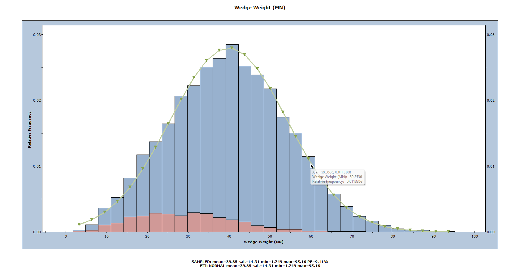
In this case, the Best Fit Distribution is a Normal distribution and the corresponding parameters are displayed at the bottom. All features of the Safety Factor histogram described above also work for this and other data types.

Before continuing, close the Wedge Weight and Safety Factor Histogram Views by clicking the X in the upper right-hand corner of each view. Also right-click in the Wedge View and select Show Mean FS Wedge from the popup menu to re-set the display to the Mean Wedge

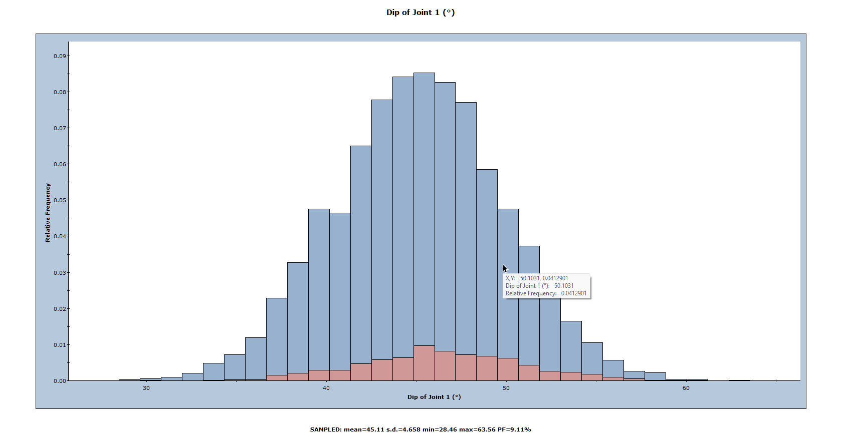
Now let’s generate a histogram of an input random variable. Re-open the Histogram Plot Parameters dialog.

1. Select: Statistics > Plot Histogram
2. Set Data Type = Dip of Joint 1.
3. Click OK.

6.3.4 Show Failed Wedges

Another feature of SWedge histogram plots is the Show Failed Wedges option. This option allows you to see the relationship between wedge failure and the distribution of any input or output variable. The option is selected by default and the distribution of failed wedges (i.e., wedges with a Factor of Safety < 1) is highlighted on the histogram.

In this case, there is not a strong correlation between wedge failure and the Dip angle of Joint 1. However, there appears to be some bias towards failure at higher dip angles, as might be expected.

6.4 SCATTER PLOTS

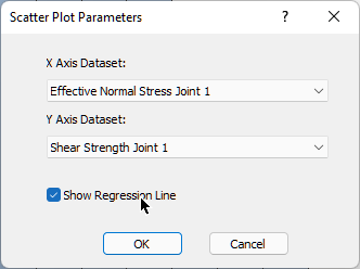
Scatter plots allow you to examine the relationship between any two analysis variables. To generate a scatter plot:

1. Select: Statistics > Plot Scatter
2. Select the variables you would like to plot on the X and Y axes (X Axis Dataset and Y Axis Dataset). For example, let's plot Effective Normal Stress and Shear Strength.
3. Select the Show Regression Line check box to display the best fit straight line through the data.
4. Click OK to generate the plot.

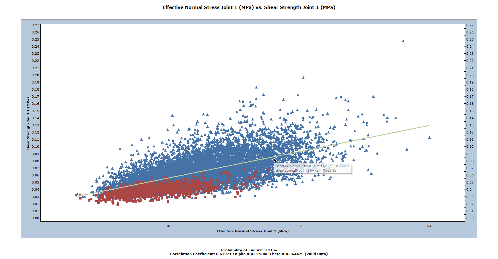
From the failed wedge data, it can be readily seen that wedge failure corresponds to low values of normal stress and shear strength, as we would expect.

Since we used the Mohr-Coulomb strength criterion, the best fit linear regression line for the scatter plot corresponds (approximately) to the mean strength envelope. We can verify this from the parameters listed at the bottom of the plot:

• The Alpha value (0.198003) represents the y-intercept of the linear regression line on the scatter plot. For Joint 1, recall that we defined the Cohesion = 0.02 MPa. For the Mohr-Coulomb criterion, cohesion is the y-intercept of the strength envelope.
• The Beta value (0.364425) represents the slope of the linear regression line. For the Mohr-Coulomb criterion, the slope of the strength envelope is equal to tan(phi). For Joint 1 we defined Phi = 20 degrees and Arctan(0.362) = 19.9.

Also note the Correlation Coefficient listed at the bottom of the plot, which indicates the degree of correlation between the two variables plotted. The Correlation Coefficient can vary between -1 and 1, where numbers close to zero indicate a poor correlation, and numbers close to 1 or –1 indicate a good correlation. Note that a negative Correlation Coefficient simply means that the slope of the best fit linear regression line is negative.

The Correlation Coefficient is related to the Coefficient of Variation, which is defined for the shear strength of Joint 1. To demonstrate this:

1. Re-open the Input Data dialog and select the Strength 1 tab.
2. Set Coefficient of Variation = 0.1 and click Apply to re-compute the analysis.
   Notice that the scatter of data around the mean strength envelope is much narrower and that the Correlation Coefficient has increased to 0.899.
3. Set Coefficient of Variation = 0.01 and click Apply again.
   Notice that the scatter of data is very narrow and that the Correlation Coefficient is 0.999.
4. To restore the original strength data, re-set Coefficient of Variation = 0.25 and click OK.

6.5 STEREONET VIEW

The Stereonet View in SWedge displays a stereographic projection of the wedge planes (great circles) and corresponding poles. For a Probabilistic analysis, the Stereonet View can display the poles of all randomly generated plane orientations as well as the joint intersections. In addition, orientations corresponding to failed wedges can be highlighted. To display the Stereonet View:

1. Select: Analysis > Stereonet
2. Right-click in the Stereonet View and make sure that the Show Planes, Show All Poles, Show Intersections, and Show Failed options are all selected. Your screen should look like the following figure:

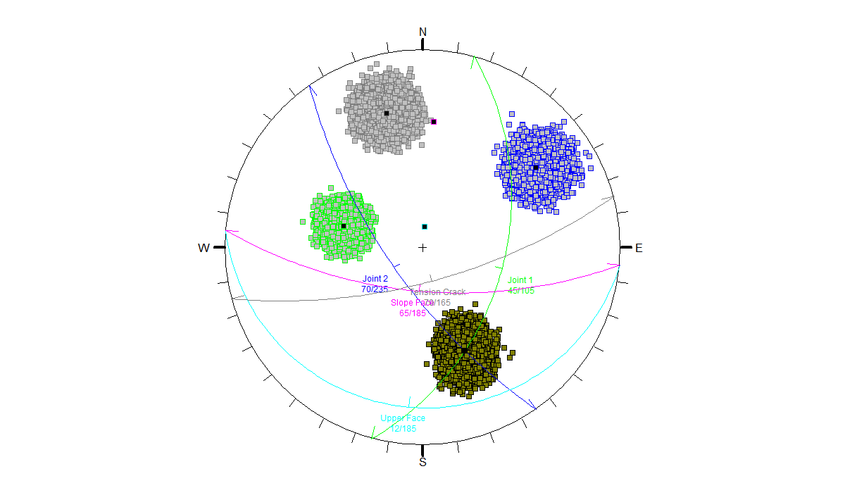
Notice the three sets of data (poles) corresponding to Joint 1, Joint 2, and the Tension Crack orientations. The set of data in the lower half of the plot represents the joint intersections, and the poles and intersections corresponding to failed wedges are highlighted in red.

6.6 COMPUTE WITH RANDOM SAMPLING

So far in this tutorial we have used the default Pseudo-Random sampling option, set as Random Number Generation in the Random Numbers tab of the Project Settings dialog (see Section 2.3 of the tutorial). Pseudo-Random sampling allows you to obtain reproducible results for a Probabilistic analysis by using the same seed value to generate random numbers. This is why you can obtain the exact values shown in this tutorial.

We will now demonstrate how different outcomes can result from a Probabilistic analysis by allowing a variable seed value to generate the random input data samples.

1. Before continuing, tile all the open views by selecting Tile on the toolbar or on the Windows menu.

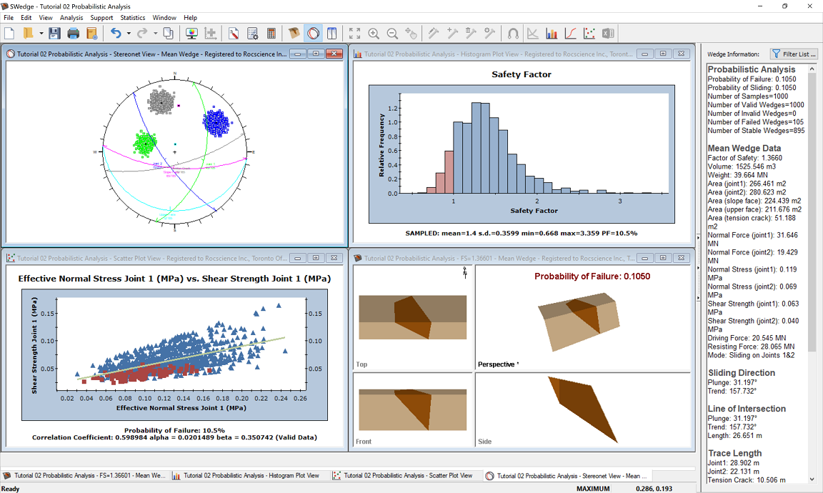
If you have followed the instructions in this tutorial, you should see four open views as shown in the following figure (Stereonet View, Histogram View, Scatter Plot View and Wedge View). You may need to decrease the font size of the plot titles and/or footers in order for them to fit in the reduced windows.

2. Right-click in the plot window, select Chart Properties , then change font settings as needed.

Now go back to the Project Settings dialog.

3. Select: Analysis > Project Settings
4. Select the Random Numbers tab.
5. Change the Random Number Generation method from Pseudo-Random to Random.
   The Random option will use a different seed value to generate random numbers each time you re-run the Probabilistic analysis. This will result in different samplings of your input random variables and different analysis results (e.g., Probability of Failure) each time you re-compute.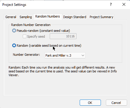
6. Select the Sampling tab and decrease Number of Samples from 10000 to 1000 to make the change easier to see on the plots.
7. Click OK.
8. Select Compute on the toolbar or on the Analysis menu.
   Notice that the plots and Probability of Failure are updated with the new results.
9. Select Compute repeatedly and observe how the plots and the Probability of Failure are updated each time the analysis is re-run.
   As you re-run the analysis, you should notice that the Probability of Failure varies between about 7% and 11%. Note also that Wedge View does not change when you re-compute since the default Mean Wedge is displayed and it is not affected by re-running the analysis.

6.7 SELECTING RANDOM WEDGES

We will again look at the ability to pick random wedges by double-clicking in either the Histogram View or the Scatter Plot View and noting the effect in the Stereonet View.

Double-click in either view repeatedly to observe the following:

• The Wedge Information Panel displays results for the Picked Wedge (the wedge that corresponds to the data location at which you clicked the plot).
• The Wedge View is updated to display the Picked Wedge.
• The great circles in the Stereonet View are updated to display the planes representing the Picked Wedge.

6.8 FILTERING BY SLIDING MODE

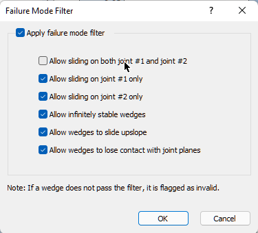
We will now look at the ability in SWedge to filter wedges by sliding mode. This feature is available in both Probabilistic and Combinations analyses. To start, open the Failure Mode Filter dialog.

1. Select: Analysis > Failure Mode Filter
2. Select the Apply failure mode filter check box to activate the filter options. By default, all filters are selected.
3. De-select Allow sliding on both joint #1 and joint # 2.
4. Click OK to apply the filters.

In this example, applying the filter produces a No Wedges are Formed message.

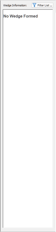
This means that all of the wedges generated in this Probabilistic analysis fail by sliding along both Joint 1 and Joint 2. We can confirm this by exporting the results to Excel and looking at the failure modes for each wedge.

To export analysis results to Excel:

1. Select Statistics > Export Dataset.
2. In the Export Statistical Datasets dialog, click the Excel button to open results in Excel.
3. Go to the Failure Mode column (the last column) and note that, for each wedge, the Failure Mode is Sliding on Joints 1 & 2.

This concludes the tutorial.