2 - Fragmentation Analysis
1.0 Introduction
This tutorial helps you become familiar with performing fragmentation analysis on a 3D model in FragMetriX’s Fragmenter tool.
The Fragmenter is a convenient tool designed for automatic particle size distribution analysis of fragmented rock. It features the delineation of single particles on a 3D model by a combined 3D surface and image analysis, the sizing of particles based on the delineated surface patches, and the determination of the particle size distribution. The fragmentation analysis runs fully automatically, and results are displayed in a particle size distribution plot and as individual delineated particles on the 3D model and on the corresponding ortho-photo. Fragmenter combines advanced 3D spatial and 2D image analysis to assess entire fragmented rock surfaces in one go and it is ideal for quarry blasting, open-pit and underground mining, tunneling, and the documentation and quality control of dams and ripraps.
Topics covered in this tutorial
- 3D Model Input
- Surface Definition
- Fragmentation Analysis
- Interpreting Results
- Editing Fragments
- Export Results
Finished product
The finished product of this tutorial, as well as all project materials, can be found in the Tutorial 2 – Fragmentation Analysis.zip folder.
2.0 Fragmenter
The Fragmenter features fast and detailed analysis and visualization of particle size distributions with its fully automated system, delivering detailed passing values and distribution functions for fragmentation assessment to provide comprehensive and objective documentation of rock masses, muck piles, and debris cones without access limitations.
It also allows to gain immediate insights into particle size distributions with color-coded visualizations of individual fragments, allowing for a quick qualitative impression of size variations without physical contact, ensuring rapid quantification of fragmented rock.
Fragmenter requires 3D models with a high-resolution topography and a high-resolution texture to ensure optimal analysis and to achieve reliable results.
Tip: The accurate determination of a particle size distribution depends on the quality of the generated surface. Input photos need to show sufficient resolution and detail to generate a high-resolution topography and a high-resolution texture 3D model. The camera used for the detection of typical rock fragments should be better than 20 megapixels with a wide angle lens camera and recorded at an altitude of about 30 m or lower.
3.0 3D Model Input
If you have not already done so, run the FragMetriX (FMX) program by:
- Double-clicking the FragMetriX icon
 on the desktop, in your installation folder or by selecting Programs > FragMetriX in the Windows Start menu.
 - When the program starts, select Fragmenter
 to run the Fragmenter tool.
When the Fragmenter tool runs, a blank project page opens as shown in the image below.
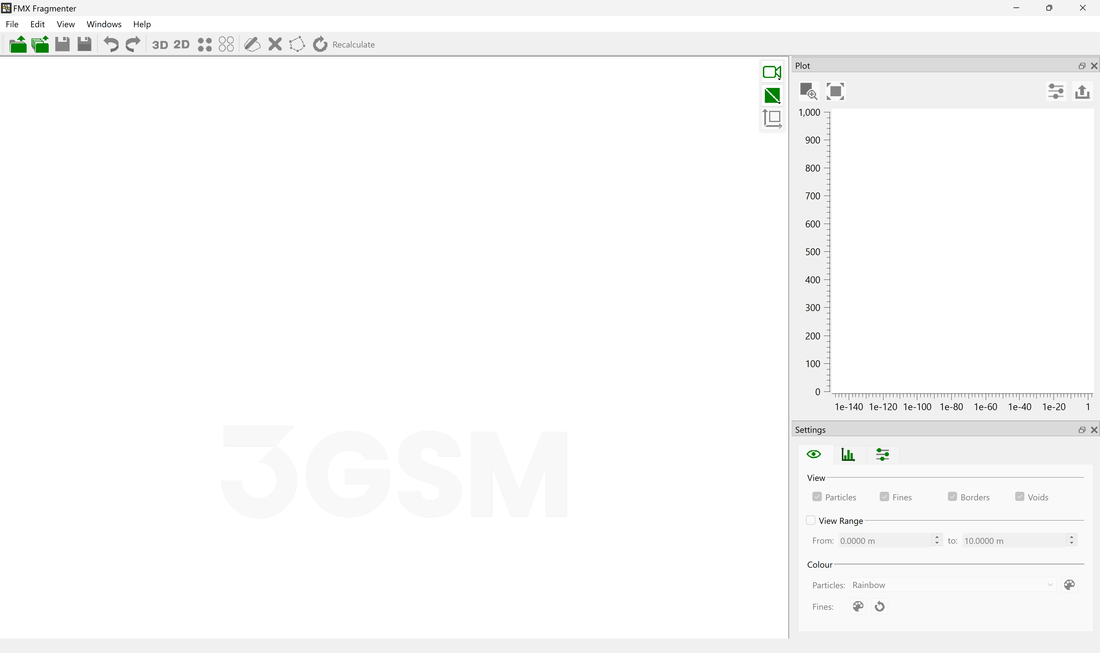
FragMetriX comes with several example images and files. These example images and files can be accessed through the Documentation> Online Resources webpage link in your FragMetriX Documentation  tool. This tutorial will use the Fragmentation Example.jm3x file generated in Tutorial 1 – 3D Model Generation to demonstrate the determination of particle size distribution features of FragMetriX.
- Select Open 3D Model

- Open the Fragmentation Example.jm3x file.
4.0 Surface Definition
The Fragmenter requires the generation of a dedicated surface for the fragmentation analysis. The generation of the surface is defined by the camera view and can be generated using one of the two options;
- Top Down – generates the surface for fragmentation analysis from the top-down camera view. This option is suitable for most of the rock fragmentation analysis surveyed by aerial imagery with Nadir (vertically downwards) flights.
- From View – generates the surface for fragmentation analysis from the current view in the 3D viewer. Requires user to align the 3D model in the 3D viewer to have an optimized view on the fragments. This option is suitable if the muck pile has a significant slope, and it was surveyed towards this particular direction (e.g. from the ground or with inclined cameras).
The surface to analyse can be limited to a certain area by defining a Region of Interest (ROI). Region of Interest is used for trimming the 3D model. To confine the fragmentation analysis to a specific region, use the analysis mask.
- Click Generate Top Down in the Open 3D Model dialog.
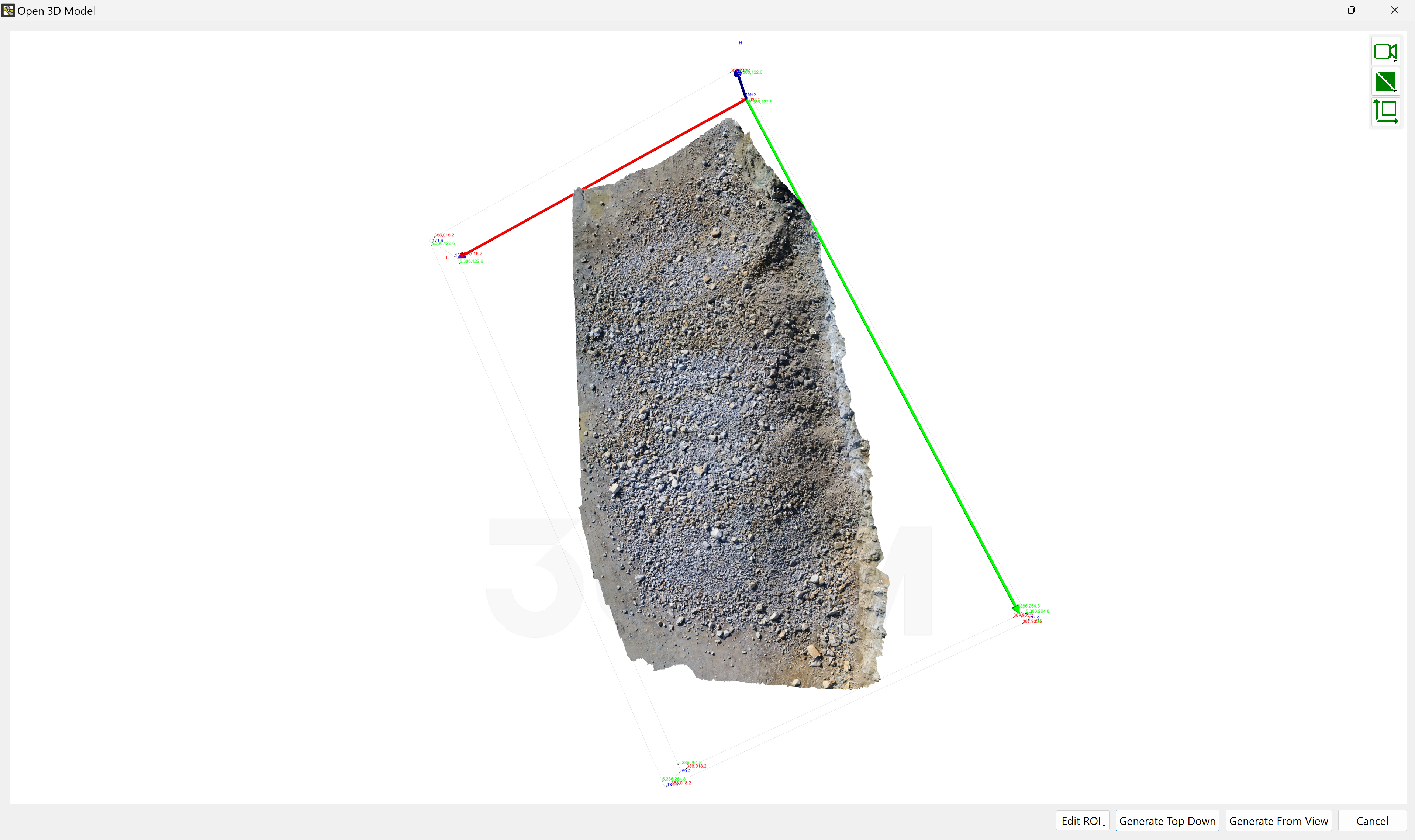
The 3D model is now imported into Fragmenter, and surface is generated for fragmentation analysis.
5.0 Fragmentation Analysis
5.1 Particle Computation Mode
Once the 3D model is opened in the Fragmenter and the surface is generated we will first need to ensure that the suitable particle computation mode is active, i.e. Blast or RipRap, in the Settings pane.
- Blast - optimized for the analysis of uniformly distributed particles (fines to boulders). A typical use case is the analysis of blasted rocks.
- Riprap - optimized for the analysis of homogenously distributed particles (a certain grain fraction). A typical use case is analysis of embankment walls and ripraps.
- Select Settings > Computation Settings

- Ensure that Blast preset is selected since we will run a fragmentation analysis on uniformly distributed particles (fines to boulders).
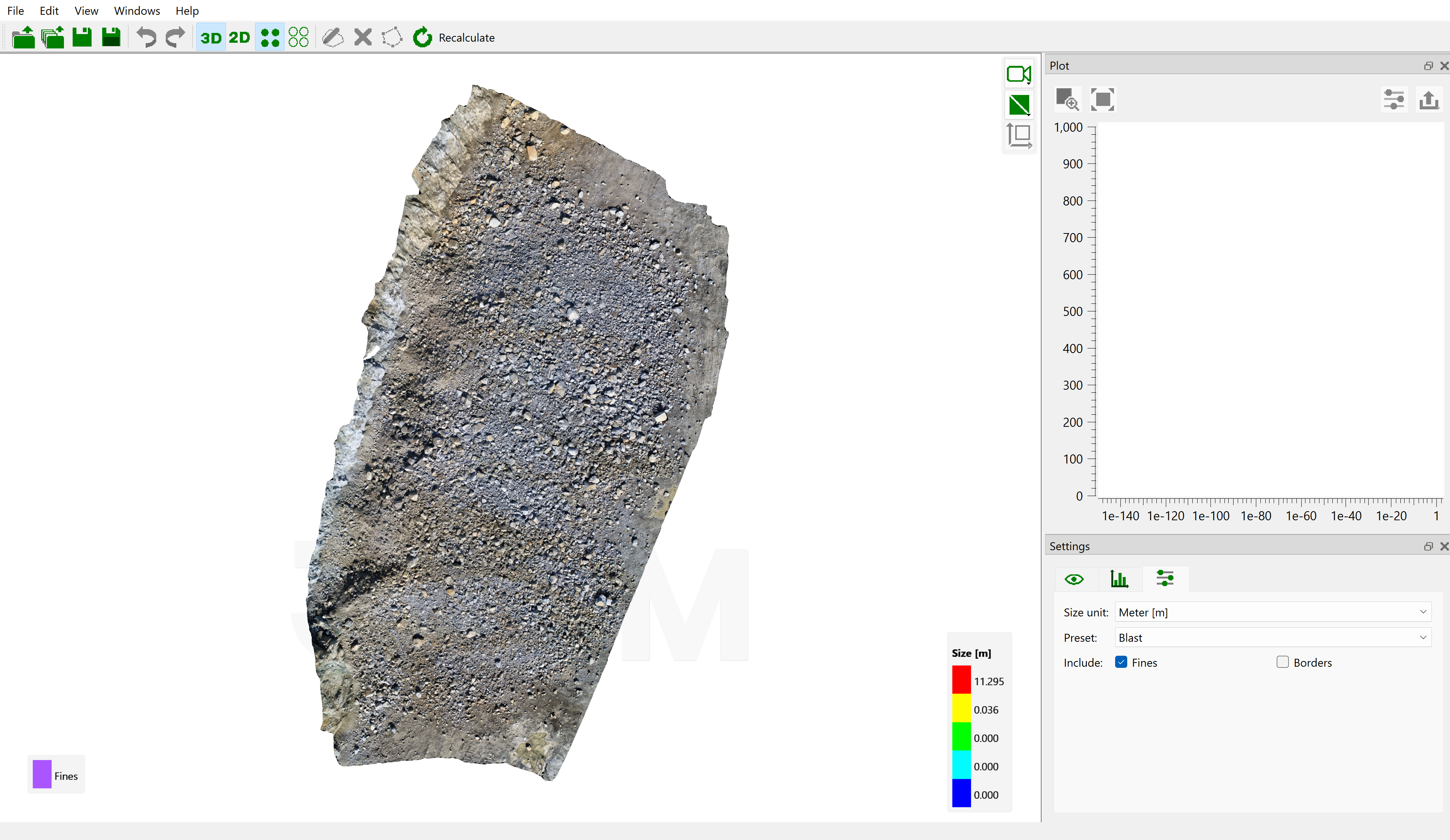
Tip: The applied particle computation mode is saved by the software and is enabled per default when opened again.
5.2 Analysis Mask
The Analysis Mask option is used to confine the fragmentation analysis to a specific area by drawing a mask. Note that the Analysis Mask is an optional feature and fragmentation analysis can be performed without defining a mask.
To draw a mask to limit the fragmentation analysis to a specific area:
- Ensure that the 2D Viewer
 is active since drawing an analysis mask is only supported in the 2D viewer.
 - Click the Draw Mask
 button in the toolbar.
 - Use your mouse to mark the border line of the mask on the image. A polygonal yellow line grows instantaneously. Undo the last selection by clicking the right mouse button, if needed.
- Confirm the polygon by pressing the Enter key or the middle mouse button.
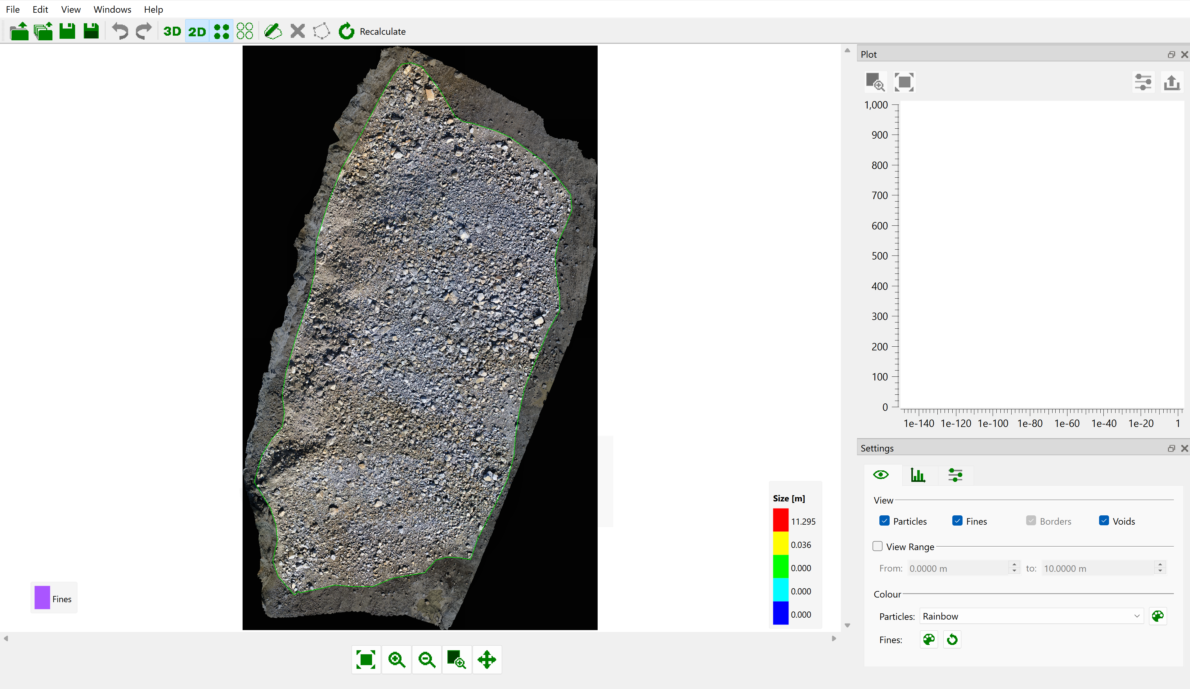
Draw an arbitrary analysis mask which includes the muck pile as shown in the below image.
5.3 Running the Fragmentation Analysis
We will now run the fragmentation analysis since we selected the suitable particle computation mode and defined the analysis mask. To run the fragmentation analysis:
- Click Recalculate

- A dialog which shows the current status of processing will appear.
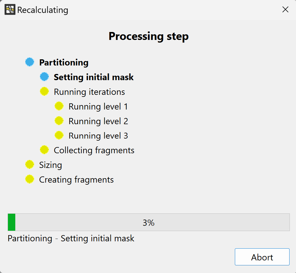
- Once the computation finishes, a colour overlay of detected fragments will be displayed in the 2D Viewer and a Particle Size Distribution Plot will be displayed in the Plot pane.
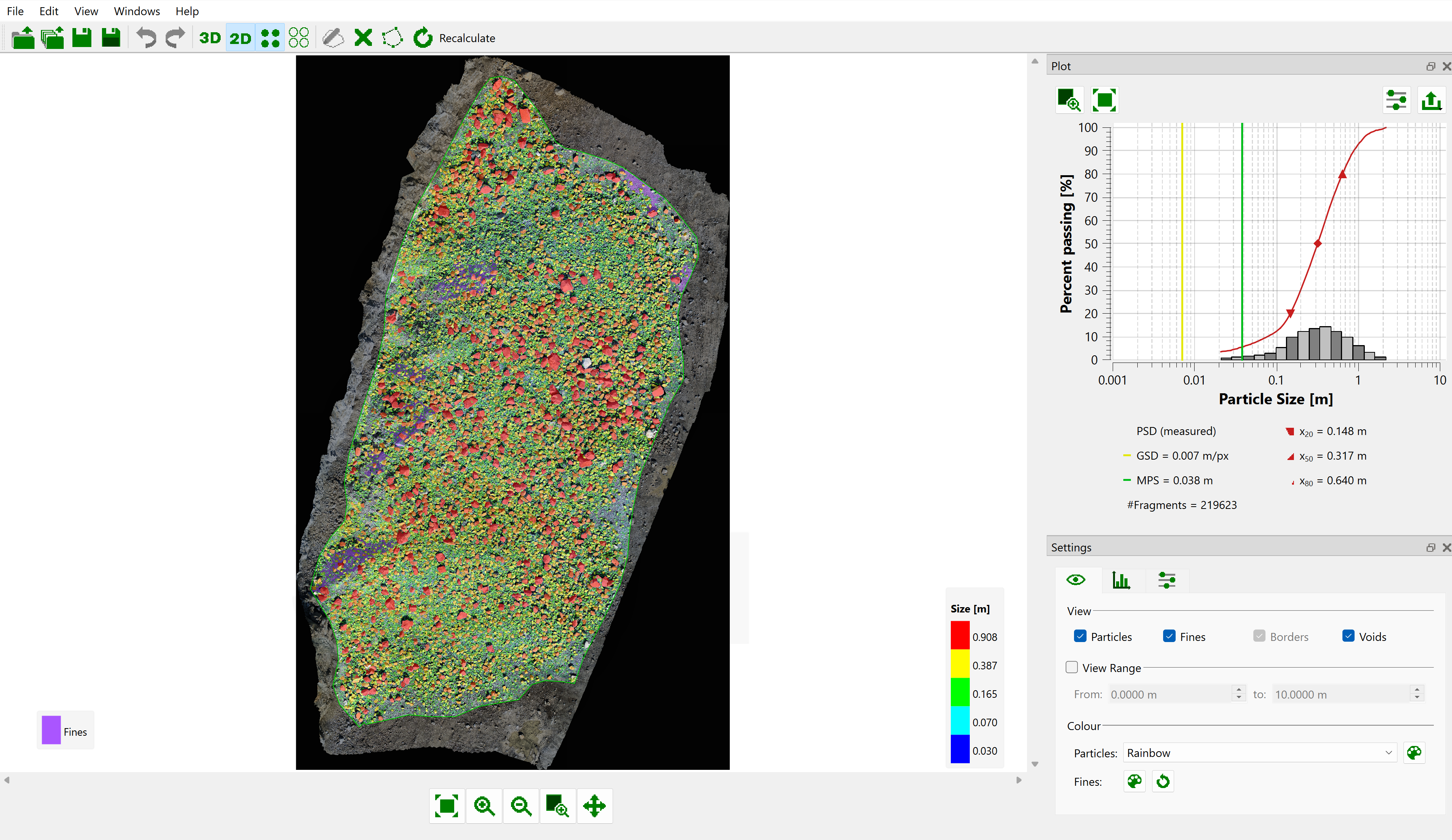
The processing time of the fragmentation analysis depends on the size of the 3D model and the computational power of the used machine.
6.0 Interpreting Results
6.1 Data Pane
The Data pane lists the detected fragments in a table. To enable the Data pane:
- Go to Windows tab and click Data.
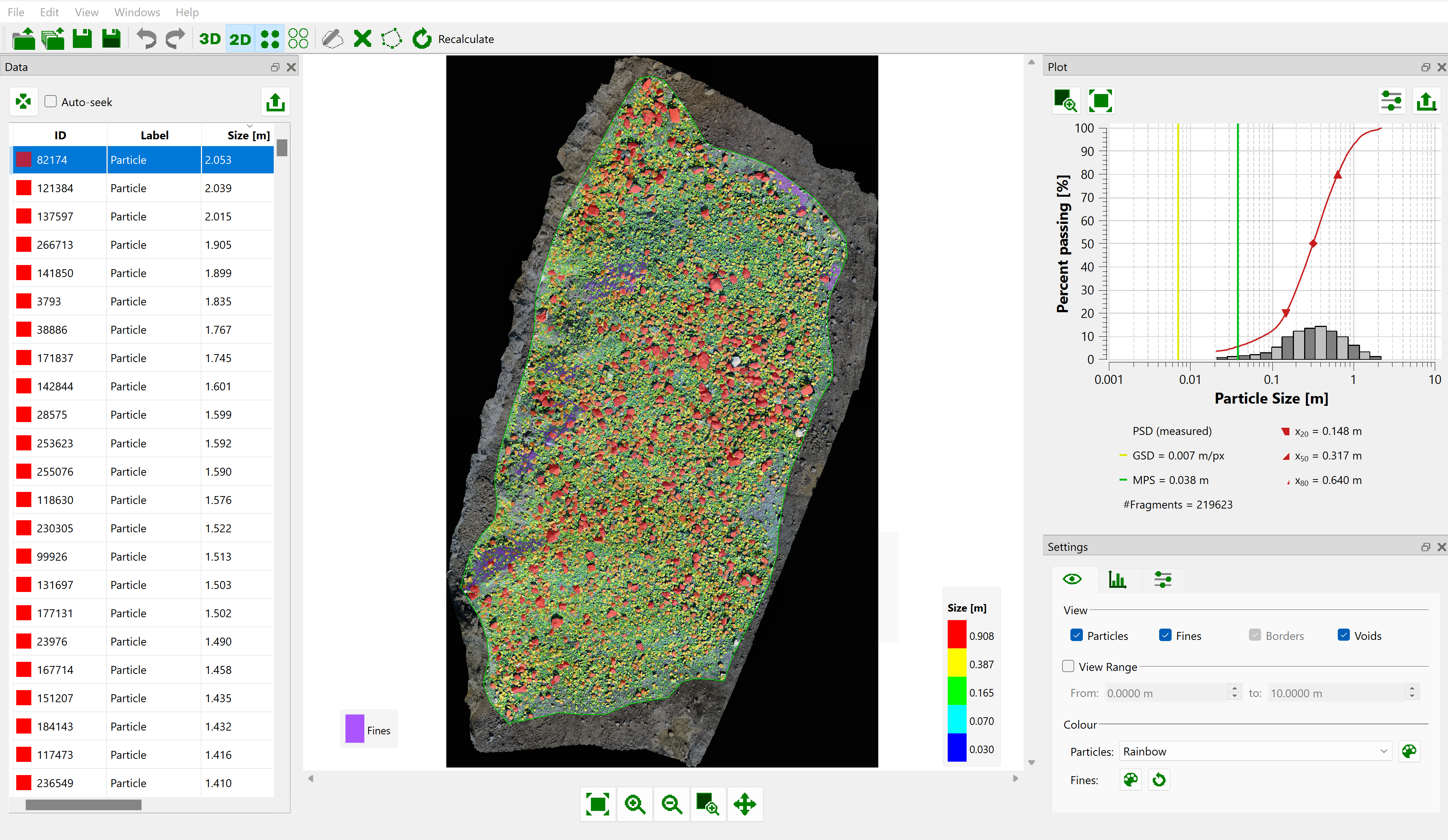
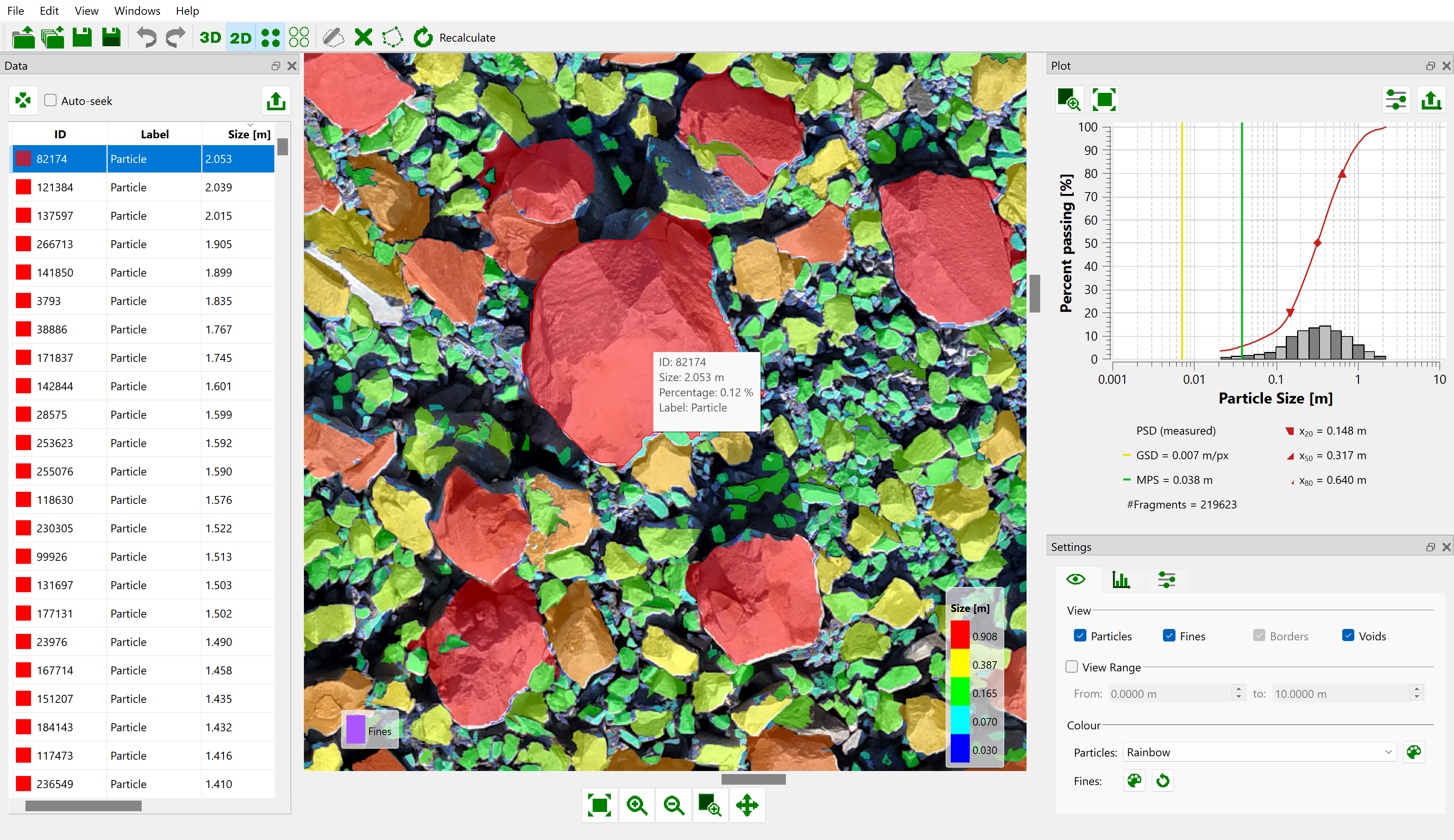
When a fragment is selected in the list, it is also highlighted in the 2D viewer with a red coloured boundary.
- The fragment is located by clicking the Seek to Fragment
 icon.
icon. - Fragments are automatically located when selected in the list by enabling the Auto-seek checkbox.
- The fragment data is exported to .csv by clicking Export Data CSV
 icon or using File > Export Data as CSV from the menu bar.
6.2 2D Viewer
The 2D surface with the corresponding color-coded overlay of fragmentation results is displayed in the 2D viewer by clicking the 2D Viewer icon in the toolbar. The legend is located at the bottom right corner of the 2D viewer. It comprises a user adjustable colour scale.
Tip: Zooming in and out can be done by Zoom In  and Zoom Out
  buttons as well as using the mouse wheel. Panning is performed by moving the mouse while keeping the middle mouse button pressed after clicking the Move
  button.
Individual fragments are selected in the 2D viewer by clicking the left mouse button on the fragment. The fragment is highlighted with a red boundary in the viewer as well as in the in the Data pane.
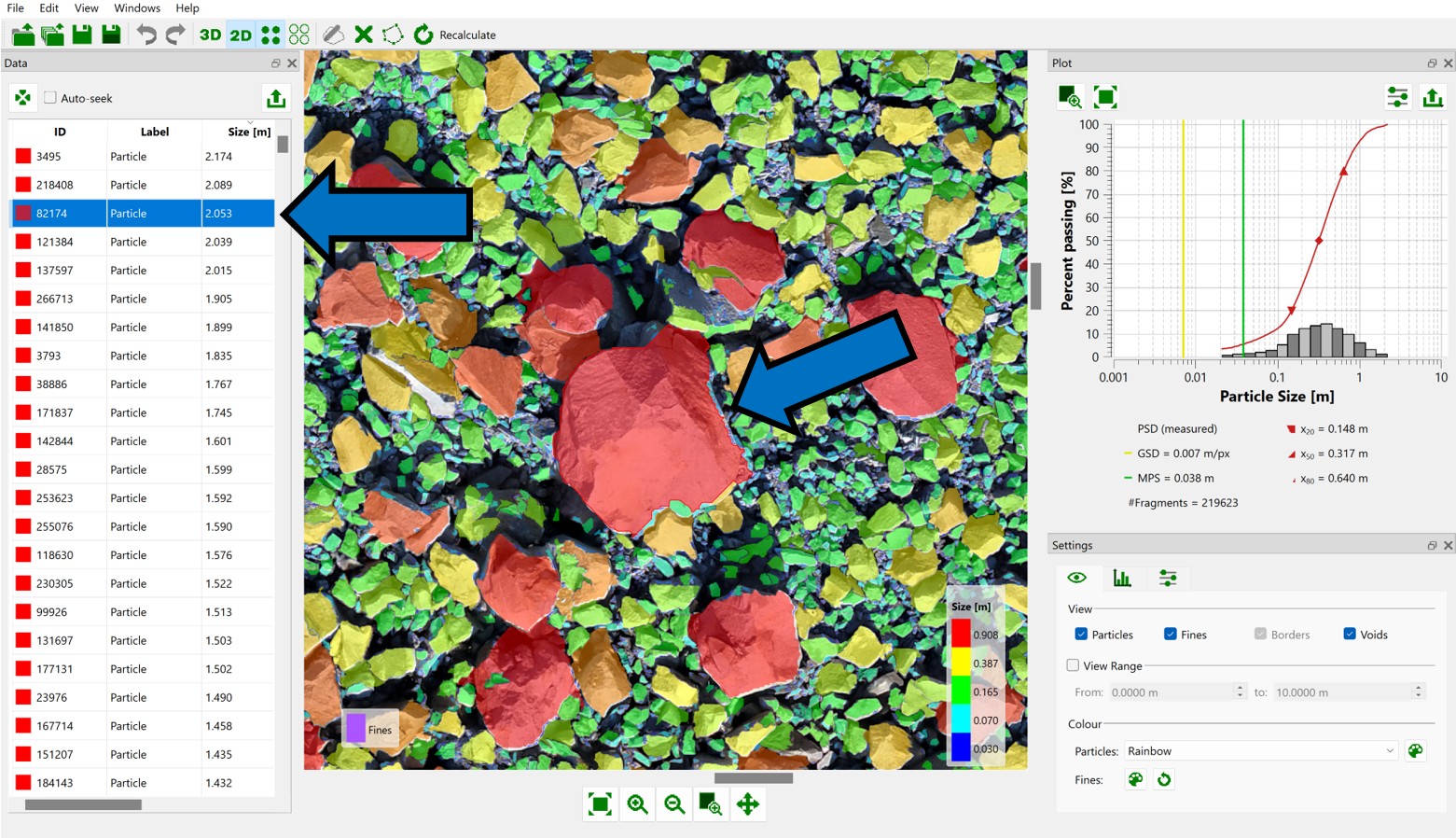
A metadata information box appears when the mouse is hovered on a fragment showing the fragment ID, the particle size, its relative percentage and assignment (label).
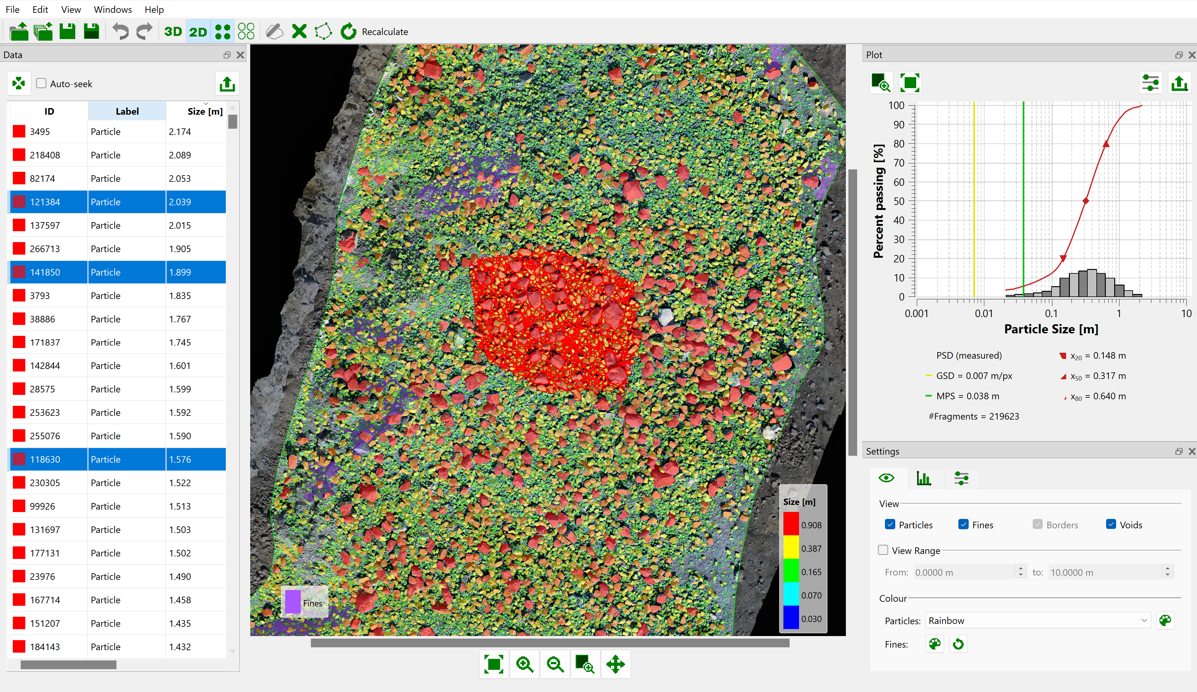
Multiple fragments are selected by enclosing the fragments by dragging the cursor while keeping the left mouse button pressed. After releasing the mouse button selected fragments are highlighted.
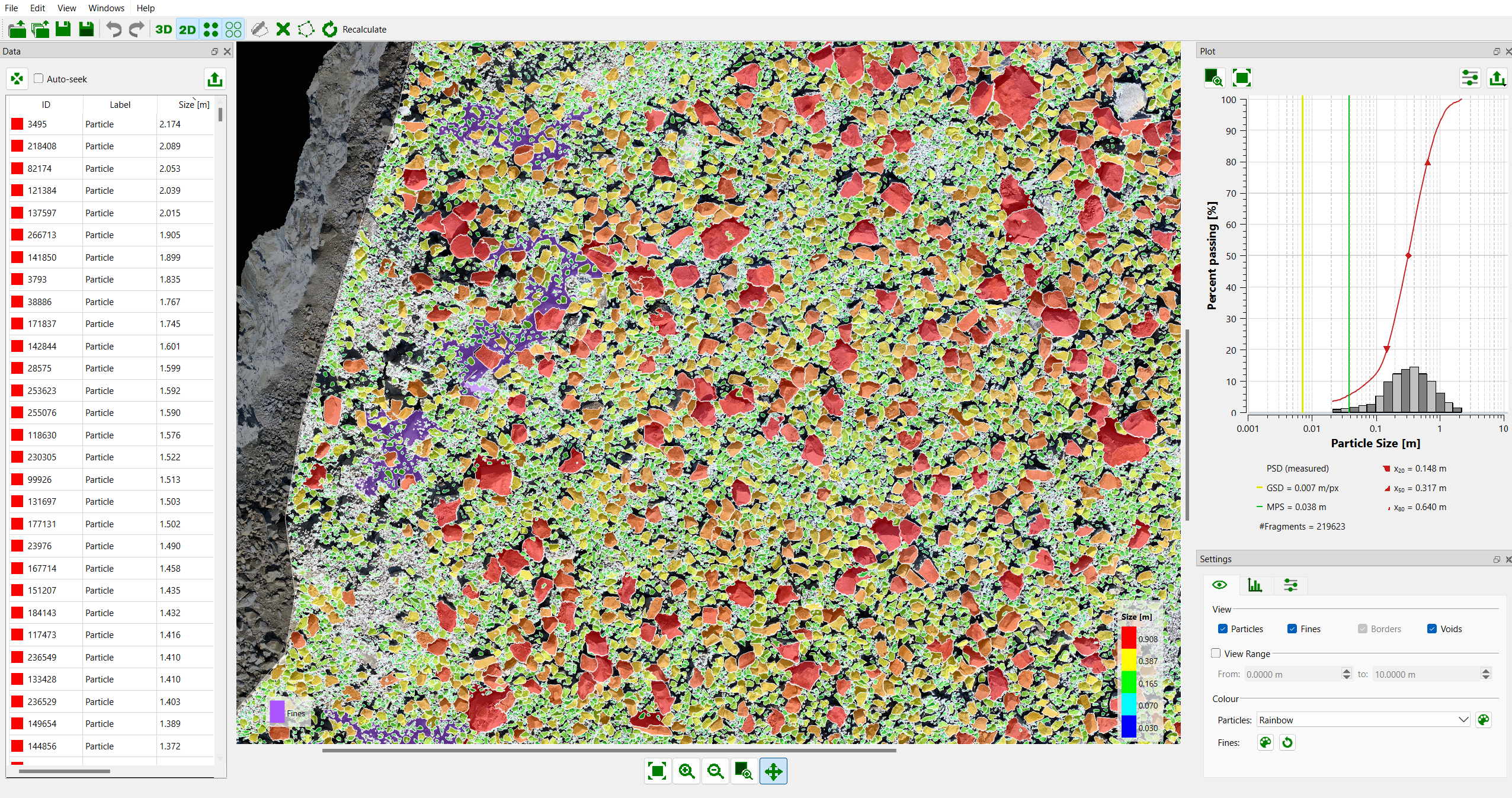
To enable/disable the display of the particle boundaries:
- Go to View > Show Particle Boundary menu or click Show Particle Boundary
 icon on the toolbar.
6.3 3D Viewer
The 3D model with the corresponding color-coded overlay of fragmentation results is displayed in the 3D viewer by clicking the 3D Viewer icon in the toolbar. The legend is located at the bottom right corner of the 3D viewer. It comprises a user adjustable colour scale.
[show particle boundary 3d]
The 3D viewer serves for visualization of fragmentation results on the 3D model only. Localization of individual fragments and editing is done in the 2D viewer.
6.4 Particle Size Distribution
The primary outcome of a fragmentation analysis is the Particle Size Distribution (PSD). The Plot Pane displays the Particle Size Distribution (PSD) curve of the detected fragments by illustrating the cumulative percentage of particles (percent passing) based on their size.
The PSD curve starts at the lower detection limit which equals to 3 times the Ground Sample Distance (GSD) of the images. Since the GSD of the current 3D model is estimated as 0.007 m/px, the lower detection limit can be calculated as 0.021m for this example.
During the imaging procedure, the minimum size of the fragments that need to be detected (xmin) should be determined first, so that the images should be captured in a way that GSD will be equal to 1/3*xmin or smaller.
Fines regions refer to areas where the photo resolution is insufficient to distinguish individual particles, or where particles cannot be identified due to low contrast or surface planarity. These regions are identified, and their percentage within the sample is calculated. This percentage is then treated as an offset in the PSD curve. In this example, fines are estimated to account for approximately 3% of the sample, causing the PSD curve to start at a percent passing value of around 3%.
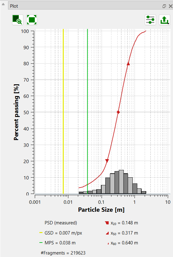
The reported X20 referring to the diameter of particles for which 20 percent of the particles are finer and 80 percent of the particles are coarser is 0.148m for this fragmentation analysis. The X50 and X80 are also reported as 0.317m and 0.640m, respectively.
The Median Point Spacing (MPS) referring to the median value of the 3D point spacing of the 3D model’s point cloud is reported as 0.038m.
Tip: The Particle Size Distribution plot grids and axes can be customized using the Plot Configuration setting.
Tip: The 2D and 3D view particle visibility, view ranges and particle colouring schemes, particle size distribution histogram settings can be customized in the Settings Pane.
To add a user-defined % passing value to the Particle Size Distribution plot:
- Go to Plot Settings tab under the Settings Pane.
- Select the User Defined Passing checkbox.
- The User Defined Passing option will be enabled. Enter the desired value to display the particle size at a user defined percentage of particles.
- Set User Defined Passing = 30% for this example.
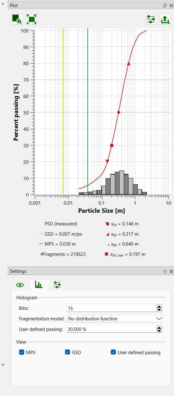
A square marker will be added in the Particle Size Distribution Plot at 30% passing value. The X30, User parameter referring to the diameter of particles for which 30 percent of the particles are finer and 70 percent of the particles are coarser is reported as 0.197m for this fragmentation analysis.
6.5 Fragmentation Model
The following best-fit fragment size distribution functions are available in FragMetriX:
- Rosin-Rammler
- Swebrec
- Swebrec Extended
To add a best-fit fragment size distribution function into Particle Size Distribution Plot:
- Go to the Plot Settings tab under the Settings Pane.
- Set Fragmentation Model = Swebrec Extended.
The selected fragmentation model is fitted in the Particle Size Distribution plot. The fitted fragmentation model parameters are listed in the Plot Pane below Particle Size Distribution plot.
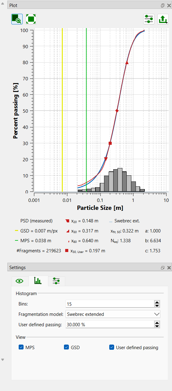
The median particle size for the best fit distribution function - Xfit,50 and degree of uniformity – Neq are reported as 0.322m and 1.338, respectively. The fitted curve shape parameters; a, b and c are also reported as 1.000, 6.634 and 1.753, respectively.
7.0 Editing Fragments
Individual fragments can be edited in the Fragmenter using the fragment editing tools in the Edit menu.
Individual fragment editing is only supported in the 2D viewer.
7.1 Merging Fragments
Multiple fragments can be merged into one using two different merging features provided in the Fragmenter:
- Merge Fragments – merges two fragments into one.
- Merge Fragments Automatically – merges several fragments into one.
To merge several fragments into one:
- Select Edit > Merge Fragments Automatically

- Select the fragments to merge by a polygon using the mouse.
- Confirm the selection by clicking the mouse wheel (middle mouse button) or pressing Enter.
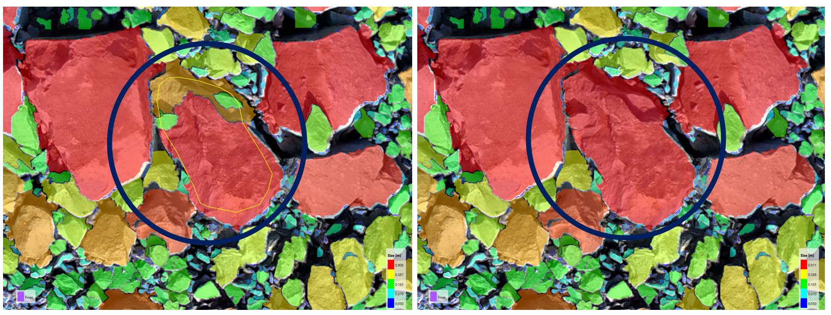
Tip: Fragments are selected if they are enclosed by the polygon or if they cross the border of the polygon.
7.2 Splitting Fragments
A single fragment can be split into two or several fragments using two different splitting features provided in the Fragmenter:
- Split Fragment – splits a fragment into two particles.
- Split Fragment Automatically – splits a fragment into several particles.
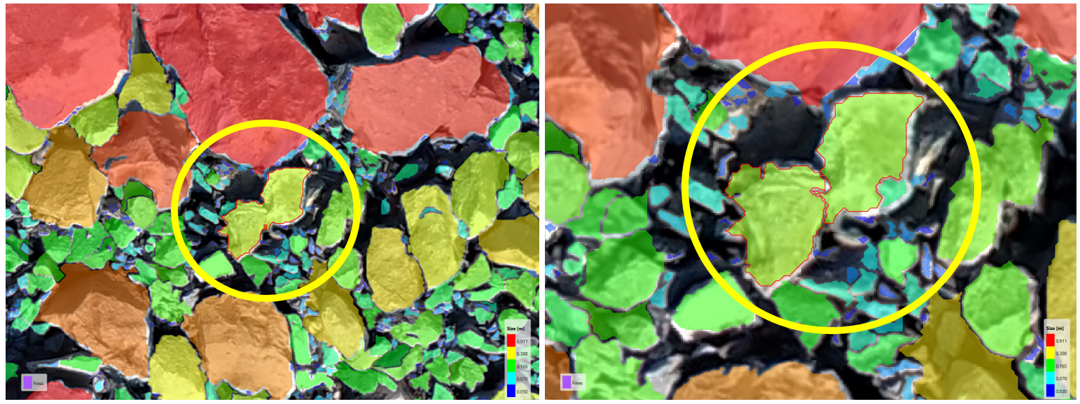
Split features consider the properties of the texture in the fragment’s texture patch and applied along the most prominent texture features of the fragment’s texture patch. To split a fragment into two:
- Select Edit > Split Fragment

- Click on two different positions in the fragment to split. To split a fragment along a particular preferred split line, click close to the preferred split line on either side.
- The Split operation will be performed after clicking the second point.
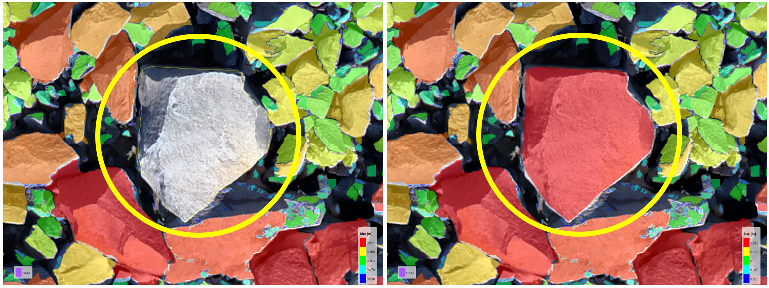
7.3 Add Fragments
To add a fragment into the analysis manually:
- Select Edit > Add Fragment

- Define the boundary of the fragment by clicking the left mouse button.
- Confirm the polygon by clicking the mouse wheel (middle mouse button) or pressing Enter.
8.0 Export Results
Fragmenter has the following options to export the Particle Size Distribution plot and the corresponding parameters.
- Export Plot as CSV
- Export Plot as PDF
- Export Data as CSV
- Export Report as PDF
To export a detailed report of the fragmentation analysis and the Particle Size Distribution plot select File > Export > Export Report as PDF.
That concludes the tutorial for Fragmentation Analysis.