7 - ShapeMetriX Import
1.0 Introduction
This tutorial demonstrates RocTunnel3’s ShapeMetriX Geometry and Joint Import options. The integration and interoperability of ShapeMetriX and RocTunnel3 streamlines the 3D block stability analysis workflow, starting from data acquisition in the field. It helps to determine each block's stability and predict failure locations and magnitudes. In this tutorial you will become familiar with importing ShapeMetriX 3D Models to generate a RocTunnel3 model and structures (i.e. joints), and using this model to perform a 3D block stability analysis.
Topics Covered in this Tutorial:
- Importing 3D Model from ShapeMetriX
- Importing Measured Joints from ShapeMetriX
- Results Interpretation
Finished Product:
The finished product of this tutorial can be found in the Tutorial 7 ShapeMetriX Integration folder, located in the Tutorials folder in your RocTunnel3 installation folder.
2.0 ShapeMetriX 3D Model Generation and Structural Mapping
ShapeMetriX is a comprehensive software suite designed for geologic mapping and geometric analysis, equipped with an advanced 3D model generator. It is ideal for creating 3D models of rock surfaces, rock slopes, tunnel faces and walls, etc. using digital imagery or by importing 3D datasets (E57 laser scanner or OBJ data) and performing fast, detailed, non-contact geological mapping and geometric assessment.
MultiPhoto, the first main component of ShapeMetriX, uses multiple overlapping images from standard drones and handheld cameras, including smartphones as input and generates 3D models by estimating the 3D structure of a scene from a set of 2D images using the Structure from Motion (SfM) process. Additionally, MultiPhoto includes standard and constrained referencing features that reference the 3D model to a higher-level coordinate system using externally surveyed Ground Control Points (GCP).
3D Model Generation and Referencing are discussed in more detail in ShapeMetriX Tutorial 1 – 3D Model Generation and Tutorial 2 – Standard and Constrained Referencing Using Ground Control Points.
Analyst, the second main component of ShapeMetriX, is a convenient tool designed for visualizing and assessing 3D models. Analyst features a fast and detailed visualization of single, multiple and merged 3D models and allows users to perform geometric measurements like dip directions and dip angles, lineaments, rock bridges (non-persistent elements), areas, distances, point locations, occurrences (water, single events), partitioning of areas (lithology and homogeneous areas), and many more, directly on a 3D model. Analyst also includes attributes like:
- Grouping measurements into Structure Sets
- Semi-automatic trace detection
- Automatic joint set clustering
- Orientation of areas and traces including stereographic projection and statistics
- Defining scanlines and mapping regions
- Automated region detection
- Lithologic region and homogenous area mapping
These help to streamline the geological and geotechnical assessment of rock faces or terrains across various scales, such as open pit mines, tunnel faces, rock slopes, drift faces, caverns, quarries, laboratory samples, and constructions like dams.
Geometric Measurements and Structural Mapping in ShapeMetriX are discussed in more detail in Tutorial 3 – Geometric Measurement and Structural Mapping.
3.0 3D Model
The model used in this tutorial is a horseshoe shaped tunnel with a width and height of approximately 13 m and 10 m, respectively. It contains measured joint surfaces and traces of known orientation, size, and location. The 3D model is generated in ShapeMetriX’s MultiPhoto tool using 27 underground images, and the structural mapping is performed in ShapeMetriX’s Analyst tool.
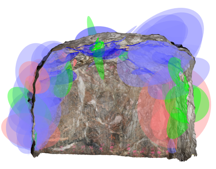
The 3D model geometry and the mapped joints data are exported as RocTunnel3 readable files (.obj for model geometry and .3gdps for joint data). These exported files will be used as input files in RocTunnel3 and can be found in the Examples > Tutorials > Tutorial 7 ShapeMetriX Integration folder in your RocTunnel3 installation folder.
3.1 Project Settings
Open RocTunnel3. You will see a blank workspace.
Our first step is to configure the analysis parameters for the model in the Project Settings.
- Select Analysis > Project Settings or click on the Project Settings
 icon in the toolbar.
 Select the Units tab.
- Set Units = Metric, stress as MPa.
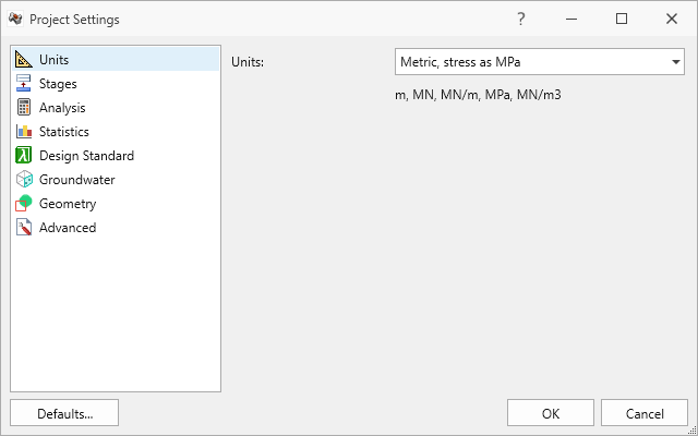
Units tab in Project Settings dialog Select the Analysis tab. Ensure:
- Design Factor of Safety = 1.0
- Successive Failure = ON
- Combined Blocks = OFF
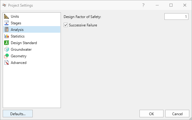
Analysis tab in Project Settings dialog - Click OK to save the settings and close the dialog.
3.2 Import Geometry
To import the Tunnel geometry into RocTunnel3:
- Select Geometry > Import/Export > ShapeMetriX Import

- In the ShapeMetriX Import dialog, click Browse , select the Tunnel Geometry.obj file in the Tutorial 7 ShapeMetriX Integration folder (located in your installation folder) and click Open.
The geometry file will be imported, and surface reconstruction will be performed automatically. The preview of the extruded volume will be displayed in the dialog.
Ensure that the Surface Reconstruction parameters are as follows:
- Shrink wrap resolution = 100
- Shrink wrap weight = 0.9
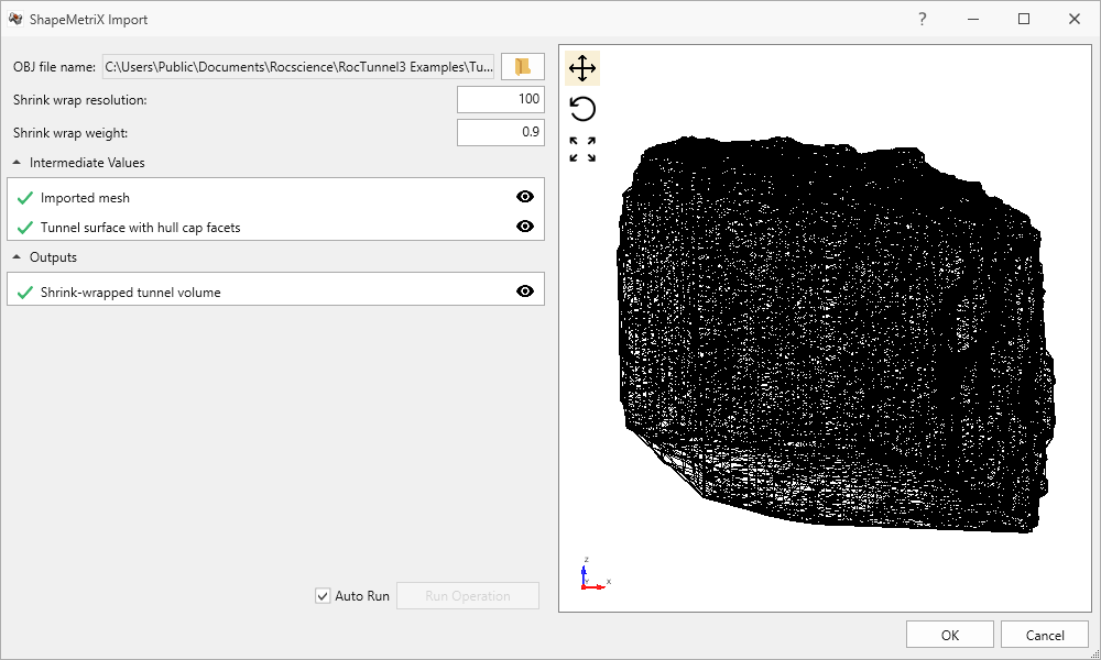
Tunnel geometry preview in ShapeMetriX Import dialog - Click OK to complete the geometry import.
Shrink wrap resolution is the triangulation density and controls the density of the reconstructed tunnel surface. A higher value means more triangles and a denser reconstructed tunnel surface.
Shrink wrap weight controls how tight the resulting surface wraps around the input mesh. A higher value means that it is more tightly wrapped.
Tip: Auto running the shrink-wrapped tunnel volume generation from reconstructed tunnel surface can be turned on and off by selecting or deselecting the Auto Run checkbox in the ShapeMetriX Import dialog.
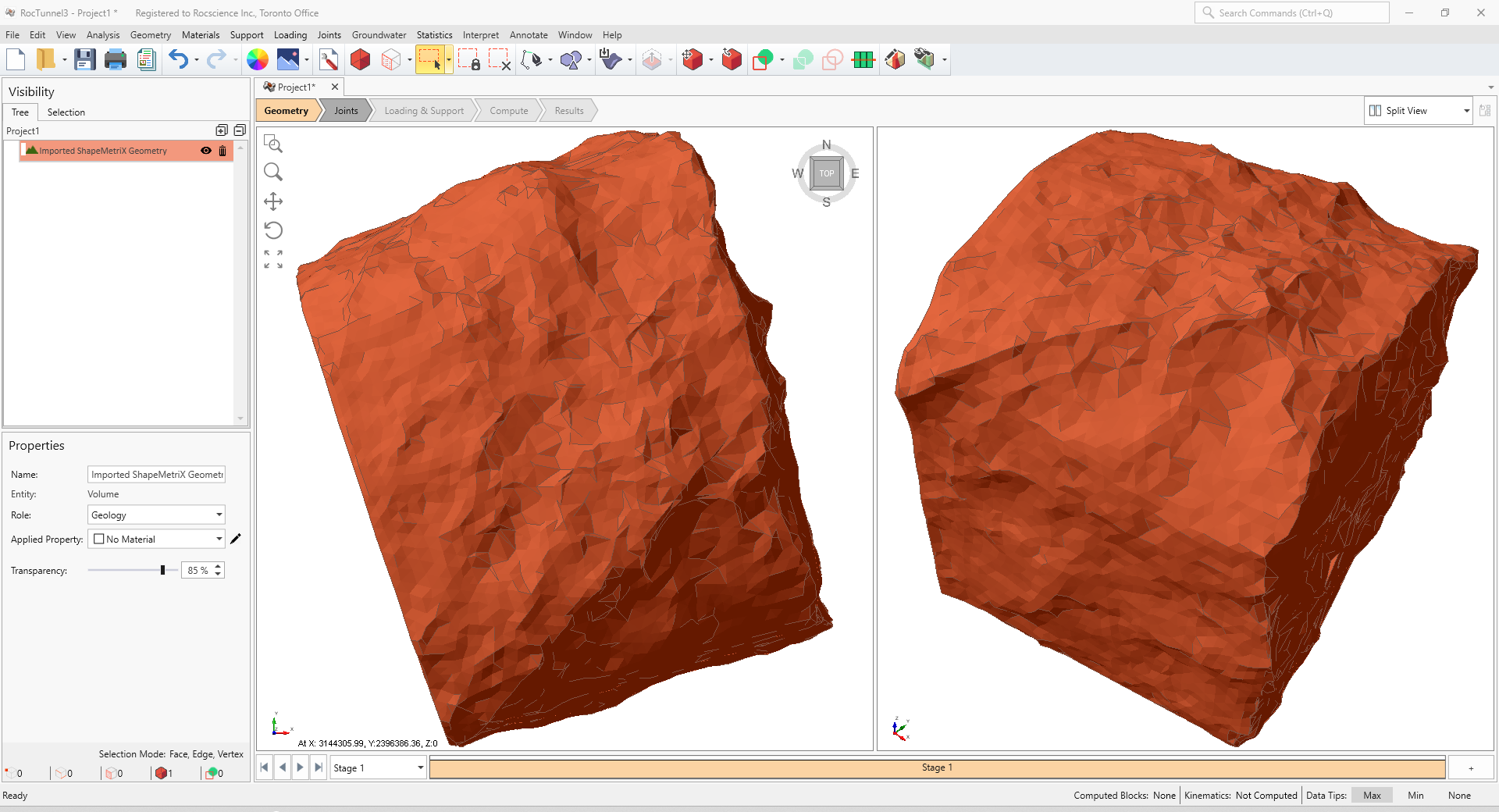
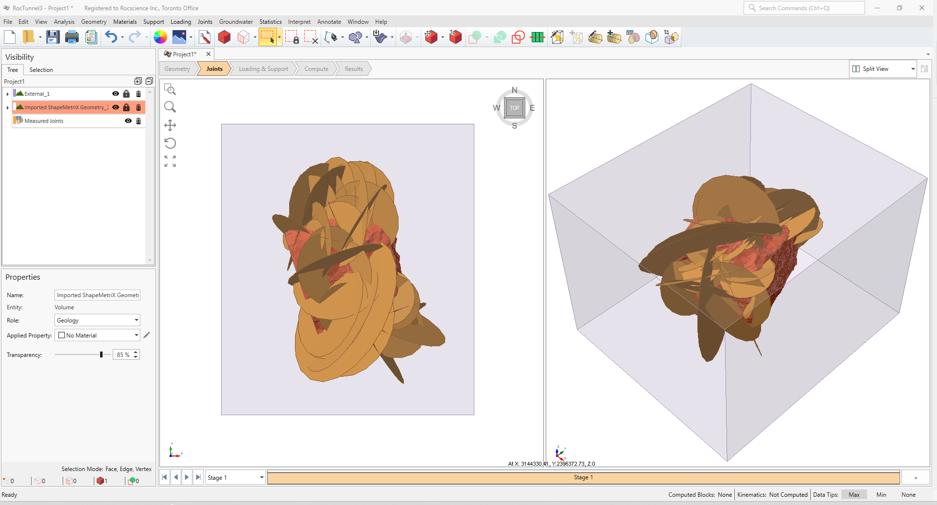
The geometry is imported into RocTunnel3 and added to the Visibility Tree.
- Select the Imported ShapeMetriX Geometry entity in the Visibility Tree.
- Assign the Imported ShapeMetriX Geometry entity as an Excavation volume in the Properties pane by setting Applied Property = No Material. The Properties pane of the Imported ShapeMetriX Geometry entity should display the following:
- Name = Imported ShapeMetriX Geometry
- Entity = Volume
- Role = Geology
- Applied Property = No Material
- Transparency = 85% (default)
3.3 Create External Volume from Box
To create a valid external for modelling, we have to define the volume which represents the rock mass surrounding the tunnel.
To create the external volume from a box:
Select Geometry > Create External Box

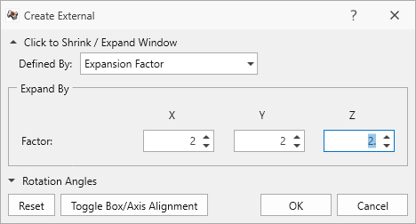
The Create External dialog allows the user to define a box as an External volume. By default, a box which bounds the entities is created. This box needs to be made bigger since blocks can only form within the rock mass.
- Set Defined By = Expansion Factor
Under Expand By enter:
- Factor X = 2
- Factor Y = 2
- Factor Z = 2
Create External dialog - Click OK to create a box and set the volume as an External.
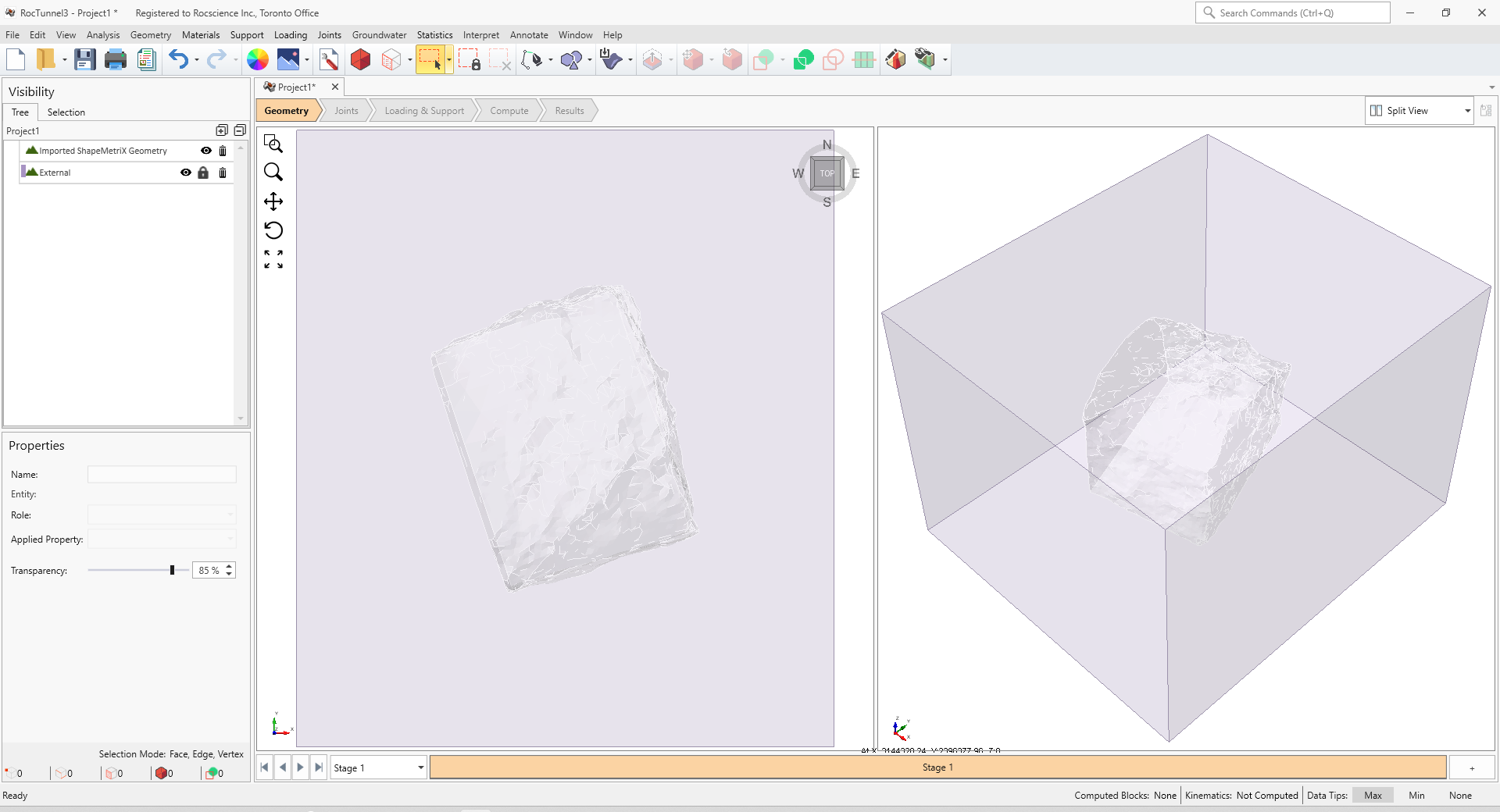
Examine the External box:
- Select the External entity in the Visibility Tree. The entity will be selected (highlighted red), and the following information is shown in the Properties pane:
- Name = External
- Entity = Volume
- Role = Geology
- Applied Property = Material 1.
- Transparency = 85%, by default
In this model, there is only one (1) Material Volume assigned with the Material 1 property.
The last step of creating the model geometry is to resolve the volume intersections so that the region within the tunnel is treated as External excavation and the region inside the box but outside the tunnel is treated as External geology.
- Select Geometry > 3D Boolean > Divide All Geometry

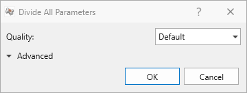
- In the Divide All Parameters dialog:
Use the default settings (Quality = Default).
Divide All Parameters dialog - Click OK.
After dividing the geometries, there are two External volumes:
- External_1 with Assigned Property = Material 1
- Imported ShapeMetriX Geometry with Assigned Property = No Material (i.e., Excavation)
3.4 Defining Joint Properties
To define joint properties:
- Navigate to the Joints
 workflow tab.
 - Select Joints > Define Joint Properties or click on the Define Joint Properties
 icon in the toolbar.
 Select Joint Property 1. Enter the following properties for Joint Property 1:
- Under the Strength tab:
- Strength Type = Mohr-Coulomb
- Cohesion = 0 MPa
- Phi = 30 deg
- Override by Material = OFF
- Waviness = 0 deg
- Under the Water Parameters tab:
- Water Pressure Method = Dry
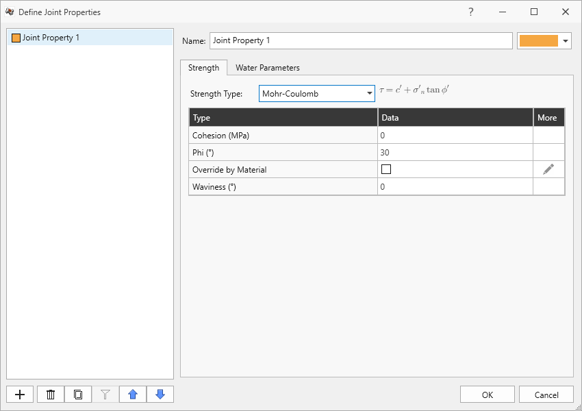
Joint Property 1 in the Define Joint Properties dialog - Under the Strength tab:
- Click OK to save and close the Define Joint Properties dialog.
3.5 Importing Measured Joints
We will be defining the joints using measured orientation data from a ShapeMetriX structural mapping file (.3gdps).
To define measured joints:
- Ensure the Joints workflow tab is still active.
- Select Joints > Define Measured Joints or click on the Define Measured Joints
 icon in the toolbar.
 - Select Shear Strength = Use Joint Properties. We will be assigning the Joint Property 1 we defined earlier.
- Click Import ShapeMetriX
- In the Open dialog, select the Tunnel Joints.3gdps file from the Tutorial 7 ShapeMetriX Integration folder and click Open.
Notice that Joint Orientations (Dip and Dip Directions), Locations (X, Y and Z) and Radius (Persistence) are imported. Joint Property 1 is also assigned to all the joints as their Joint Property.
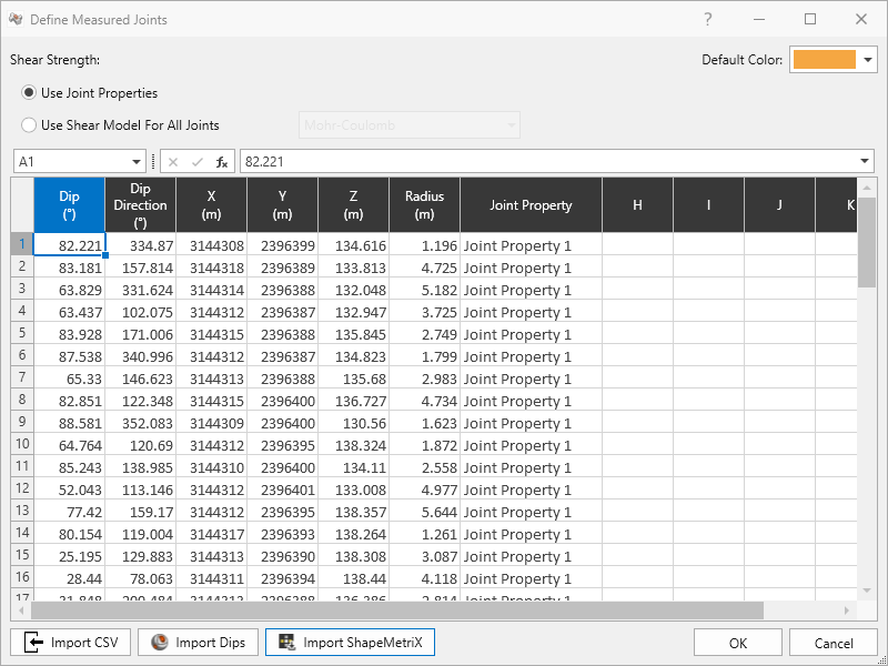
67 Joints imported in Define Measured Joints dialog - Click OK to save the inputs, exit the Define Measured Joints dialog and add the joints to the model.
4.0 Compute
RocTunnel3 has a two-part Compute process.
4.1 Compute Blocks
The first step is to compute the unit blocks which may potentially be formed by the intersection of joints with other joints and the intersection of joints with the free surface.
To compute the unit blocks:
- Navigate to the Compute
 workflow tab.
 - Select Analysis > Compute Blocks

As compute is run, the progress bar reports the compute status. Once compute is finished, the Results node is added to the Visibility Tree and All Valid Unit Blocks are shown in the 3D View. The Results node consists of the collection of valid unit blocks and the socketed excavation. The original External and Measured Joints visibility is turned off.
Once compute is finished, the unit blocks are colored according to the Block Color option (Random Colors) set in the Results node's Properties pane.
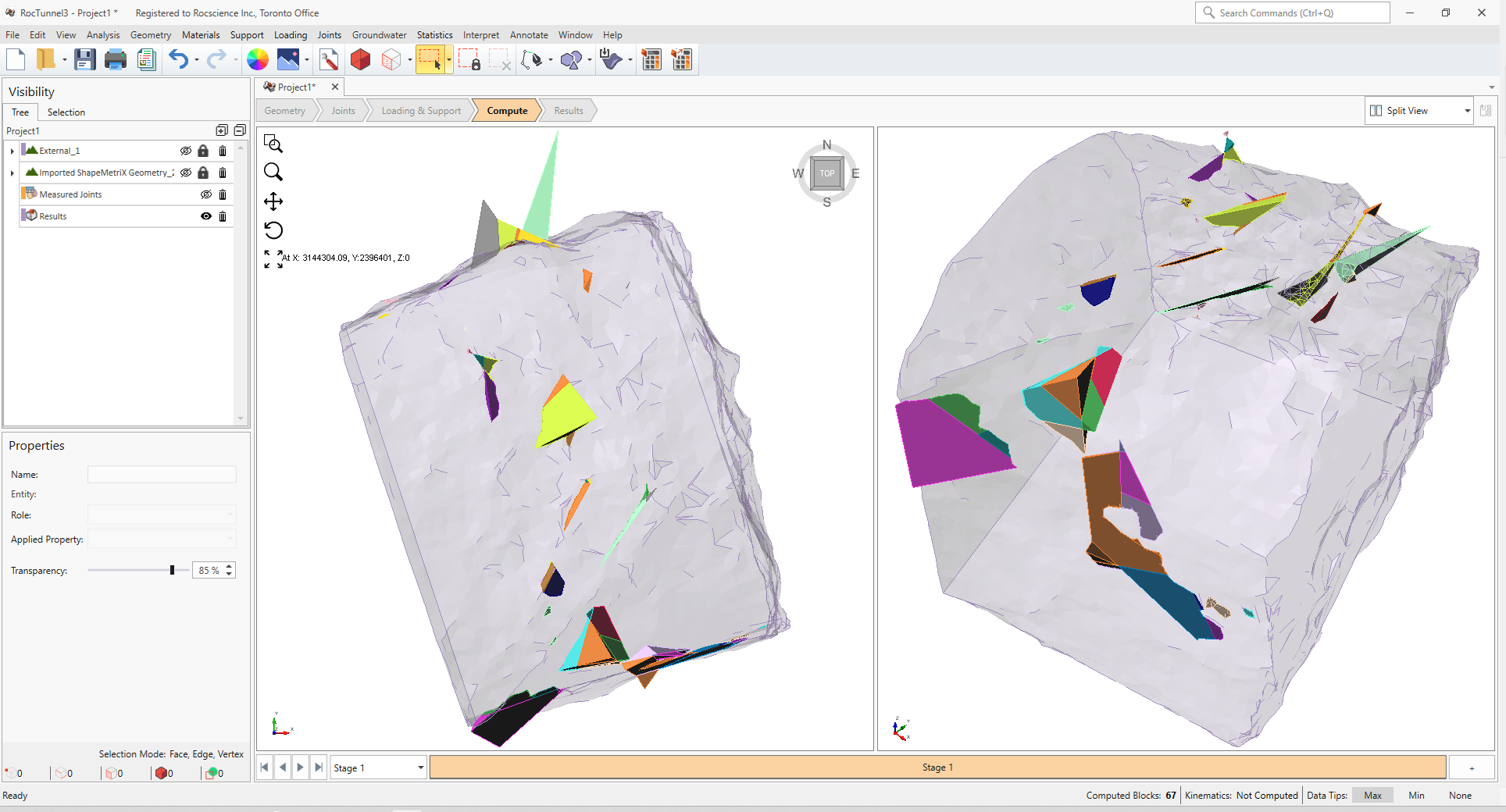
Compute Blocks only determines the geometry of the unit blocks. In order to obtain other information such as the factor of safety, Compute Kinematics needs to be run.
4.2 Compute Kinematics
The second and final compute step is to compute the removability, forces, and factor of safety for each of the valid unit blocks.
To compute the block kinematics:
- Ensure that the Compute workflow tab is still the active workflow.
- Select Analysis > Compute Kinematics or click the Compute Kinematics
 icon in the toolbar.
As compute is run, the progress bar reports the compute status. By default, after Compute Kinematics is run, only Removable Unit Blocks are shown.
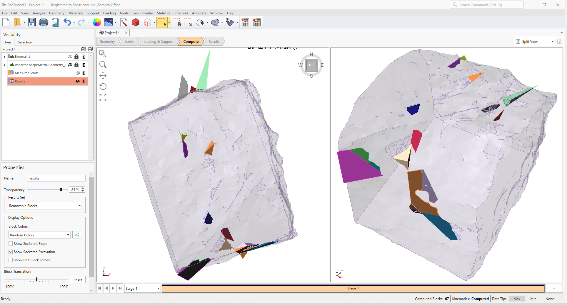
In a Successive Failure mode of analysis, several Failure Iterations may be performed. In the first Failure Iteration, only immediately removable daylighting unit blocks are analyzed. Any unit blocks which have a factor of safety less than the Design Factor of Safety (set in Project Settings) is considered "failed". These unit blocks are also known as "key blocks". The stability of key blocks controls the global stability of the slope. As key blocks fail and are detached from the slope, potential constraints in joint faces (in regard to removability and valid sliding direction) are removed and become free faces which no longer support the block or provide shear resistance to sliding. As such, the failure proceeds in a successive manner. See the Analysis topic for more information on Successive Failure.
Successive Failure analysis in RocTunnel3 is currently only applicable to unit blocks and does not model the interaction between unit blocks; the unraveling mechanism is much more complex. Instead, RocTunnel3 looks at each unit block in isolation during each Failure Iteration.
5.0 Interpreting Results
Once both blocks and kinematics are computed, all block results can be viewed in a grid format.
- Select the Results
 workflow tab.
 - Select Interpret > Block Information or click on the Block Information
 icon in the toolbar to view the Block Information Grid.
5.1 Failed Unit Blocks
To view failed unit blocks:
- Select the Results node from the Visibility Tree
- Set Results Set = Failed Unit Blocks (FS < Design FS)
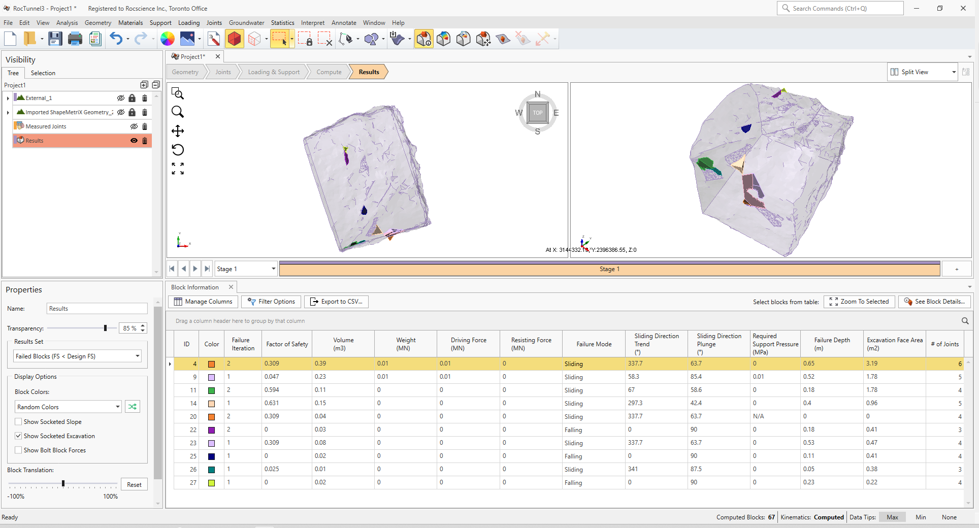
Of the 67 valid unit blocks that formed, only 10 of them are flagged as failed unit blocks with Factor of Safety less than the Design Factor of Safety of 1.
This concludes Tutorial 07.