4 - Probabilistic Analysis
1.0 Introduction
In a Probabilistic Analysis, statistical input data can be entered to account for uncertainty in material unit weight, joint shear strength, and joint water pressure. The result is a distribution of factors of safety, from which probability of failure is calculated for any given block formed from a single realization of the joint geometry (i.e., geometry of the blocks are deterministic across all sample runs; only material and joint property parameters are used as random variables).
Finished Product
The finished product of this tutorial can be found in the Probabilistic Analysis.roctunnel_model file. All tutorial files installed with RocTunnel3 can be accessed by selecting File > Recent Folders > Tutorials Folder from the RocTunnel3 main menu.
2.0 Opening the Starting File
- Select File > Recent > Tutorials Folder.
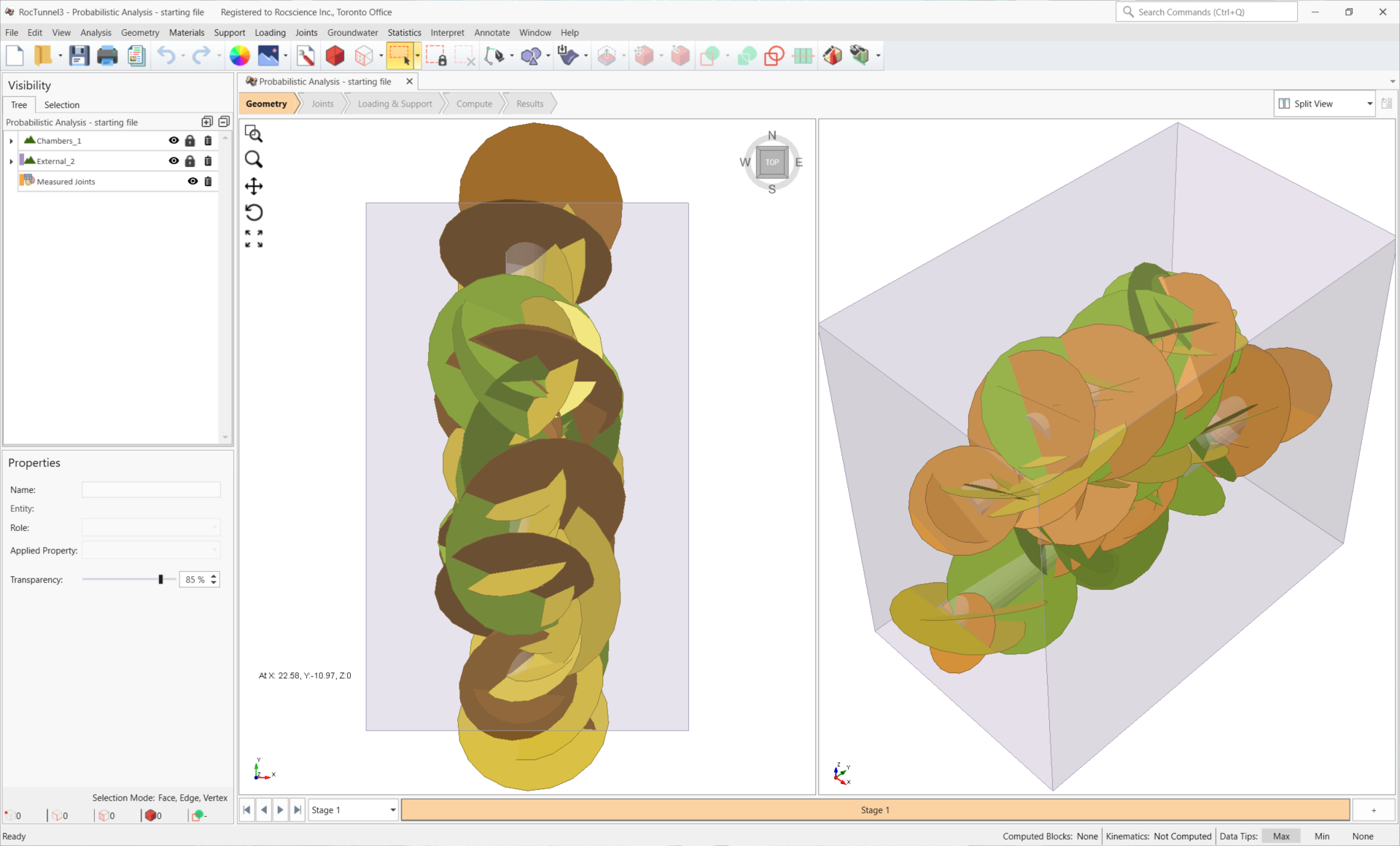
- Go to the Tutorial 04 Probabilistic Analysis folder, and open the file Probabilistic Analysis - starting file.roctunnel_model.
This model already has the following defined and provides a good starting point to start computing blocks:
- Deterministic Material Properties
- External Geometry
- Deterministic Joint Properties
- Measured Joints
2.1 Project Settings
Our first step is to configure the Statistics settings for the model in Project Settings.
- Select Analysis > Project Settings

- Select the Units tab.
Ensure Units are Metric, stress as MPa.
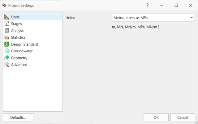
Units tab in Project Settings dialog
- Select the Analysis tab.
- Set Design Factor of Safety = 1.5.
- Ensure Successive Failure is ON. When Successive Failure is ON, blocks which are exposed on the excavation are analyzed first followed by any subsequent blocks which may become unstable due to the failure and removal of neighboring key blocks.
- Ensure Combined blocks is OFF. We will only be looking at unit blocks in this tutorial.
- Select the Statistics tab.
- Select Probabilistic Analysis to turn on probabilistic analysis mode.
Leave the default Sampling Method = Latin-Hypercube and default Number of Samples = 1000
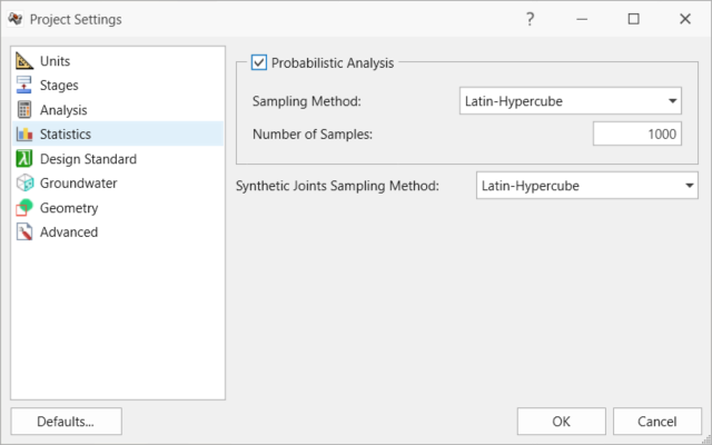
Statistics tab in Project Settings dialog
- Click OK to save the settings and close the dialog.
2.2 External Geometry
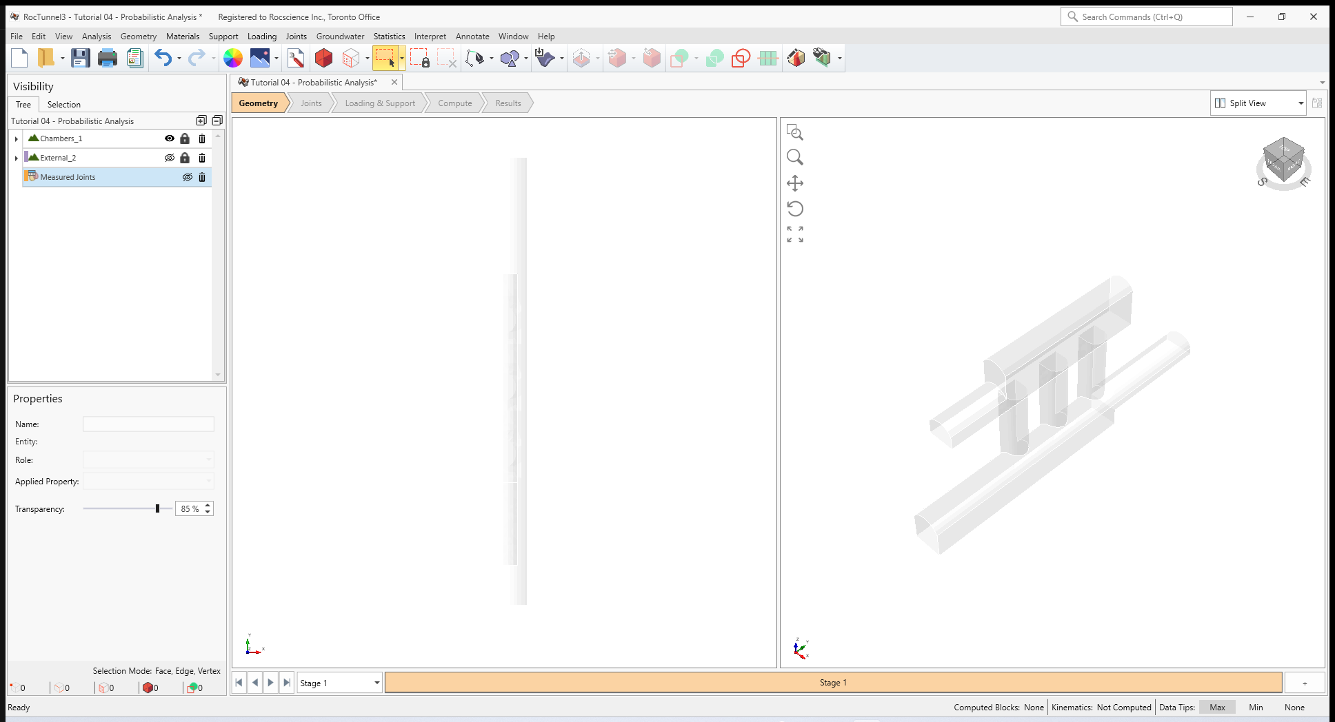
The External is of a two tunnel drives, meeting at a junction (i.e., the excavation assigned "No Material") and bounded by a box volume assigned with Material 1 material property. The Material 1 material property is currently defined as deterministic.
To see only the Excavation entities:
- Select the External_2 node's Visibility icon to turn off the node's visibility
- Select the Measured Joints node's Visibility icon to turn off the node's visibility
2.3 Joint Surfaces
Review the Measured Joints.
- Select Joints > Define Measured Joints

57 Measured Joints are defined and listed in order of Dip, Dip Direction, X, Y, Z, Radius, and Joint Property:
| Dip | Dip Direction | X | Y | Z | Radius | Joint Property |
| 26 | 147 | 94 | -13 | 928 | 25 | Set 1 |
| 20 | 130 | 95 | -10 | 928 | 13 | Set 1 |
| 28 | 183 | 100 | 8 | 928 | 24 | Set 1 |
| 48 | 175 | 93 | 13 | 939 | 15 | Set 1 |
| 37 | 156 | 100 | 33 | 939 | 24 | Set 1 |
| 29 | 234 | 93 | 51 | 939 | 24 | Set 1 |
| 39 | 223 | 93 | 58 | 939 | 22 | Set 1 |
| 32 | 179 | 95 | 63 | 939 | 11 | Set 1 |
| 50 | 194 | 99 | 66 | 939 | 12 | Set 1 |
| 38 | 196 | 103 | -26 | 888 | 14 | Set 1 |
| 51 | 222 | 94 | 32 | 888 | 11 | Set 1 |
| 28 | 193 | 96 | 41 | 888 | 11 | Set 1 |
| 37 | 235 | 103 | 48 | 888 | 12 | Set 1 |
| 51 | 190 | 96 | 101 | 888 | 19 | Set 1 |
| 21 | 213 | 100 | 115 | 888 | 12 | Set 1 |
| 28 | 153 | 100 | 22 | 915 | 15 | Set 1 |
| 59 | 201 | 91 | 21 | 908 | 22 | Set 1 |
| 36 | 193 | 93 | 22 | 894 | 12 | Set 1 |
| 51 | 223 | 99 | 43 | 922 | 16 | Set 1 |
| 29 | 99 | 95 | 23 | 939 | 12 | Set 2 |
| 25 | 92 | 93 | 41 | 939 | 24 | Set 2 |
| 38 | 119 | 100 | 51 | 939 | 12 | Set 2 |
| 55 | 55 | 93 | 71 | 939 | 16 | Set 2 |
| 20 | 68 | 92 | 73 | 939 | 18 | Set 2 |
| 45 | 38 | 96 | 79 | 939 | 10 | Set 2 |
| 32 | 100 | 101 | -4 | 888 | 24 | Set 2 |
| 45 | 51 | 103 | 24 | 888 | 12 | Set 2 |
| 51 | 99 | 100 | 36 | 888 | 13 | Set 2 |
| 28 | 13 | 101 | 63 | 888 | 11 | Set 2 |
| 49 | 28 | 101 | 82 | 888 | 20 | Set 2 |
| 49 | 21 | 95 | 21 | 896 | 14 | Set 2 |
| 57 | 61 | 91 | 22 | 894 | 24 | Set 2 |
| 33 | 105 | 97 | 43 | 915 | 19 | Set 2 |
| 28 | 64 | 97 | 43 | 913 | 11 | Set 2 |
| 20 | 53 | 94 | 43 | 894 | 18 | Set 2 |
| 56 | 334 | 100 | -5 | 928 | 23 | Set 3 |
| 33 | 316 | 96 | -3 | 928 | 21 | Set 3 |
| 33 | 288 | 98 | 3 | 928 | 22 | Set 3 |
| 25 | 357 | 100 | 5 | 928 | 11 | Set 3 |
| 33 | 260 | 100 | 13 | 928 | 14 | Set 3 |
| 25 | 281 | 99 | 13 | 933 | 22 | Set 3 |
| 50 | 347 | 92 | 21 | 939 | 23 | Set 3 |
| 44 | 306 | 96 | 28 | 939 | 17 | Set 3 |
| 43 | 291 | 96 | 36 | 939 | 15 | Set 3 |
| 24 | 351 | 91 | 46 | 939 | 15 | Set 3 |
| 51 | 299 | 96 | 68 | 939 | 18 | Set 3 |
| 24 | 321 | 100 | 73 | 939 | 13 | Set 3 |
| 38 | 260 | 100 | 79 | 939 | 22 | Set 3 |
| 25 | 345 | 98 | -23 | 888 | 23 | Set 3 |
| 45 | 306 | 101 | -16 | 888 | 12 | Set 3 |
| 30 | 310 | 97 | 74 | 888 | 16 | Set 3 |
| 56 | 280 | 97 | 86 | 888 | 17 | Set 3 |
| 46 | 289 | 95 | 96 | 884 | 24 | Set 3 |
| 53 | 265 | 96 | 22 | 922 | 25 | Set 3 |
| 38 | 341 | 100 | 22 | 920 | 25 | Set 3 |
| 33 | 250 | 91 | 21 | 901 | 16 | Set 3 |
| 21 | 7 | 99 | 43 | 917 | 18 | Set 3 |
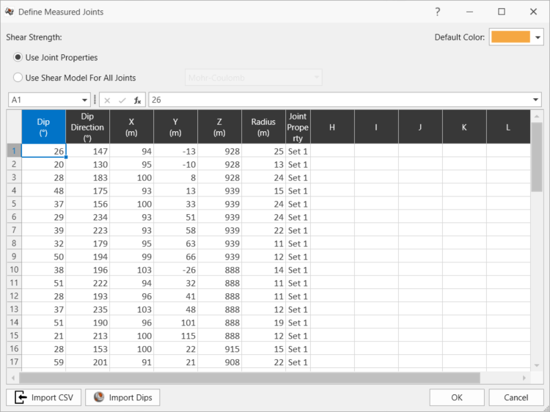
- Click OK to close the dialog.
All joint properties in Set 1, Set 2, and Set 3 are currently defined as deterministic.
3.0 Random Variables
In order to run a Probabilistic Analysis, at least one random variable must be defined and used in the model. In RocTunnel3, the following can be set as a random variable:
Material Property parameters (e.g., Unit Weight, Ru Value)
The availability of random variables depends on the Groundwater Method selected.Joint Property parameters (e.g., Cohesion, Phi, Waviness, Uniform Water Pressure)
The availability of random variables depends on the Strength Type and Water Pressure Method selected.
For this model, we will be modelling the variability in Unit Weight of the material and the Friction Angle of shear strength properties of the joints.
3.1 Material Property Statistics
To assign statistics to Material Properties:
- Select: Materials > Define Materials
 . The Define Materials dialog shows the mean parameter values of Material 1:
- Ensure Unit Weight = 0.026 MN/m3
No Water Surface is applied.
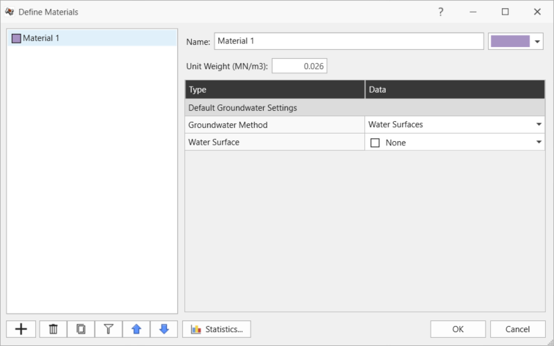
Deterministic values of Material 1 material property in Define Materials dialog
Select the Statistics button.
The Define Material Statistics dialog allows users to add any applicable inputs as random variables. Only one Material Property exists (i.e., Material 1).
The Define Material Statistics dialog can also be accessed in Statistics > Define Material Statistics.- Click the Add button.
- In the Add Random Variables dialog:
Select Unit Weight.
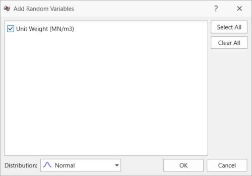
Add Random Variables dialog - Click OK. The Unit Weight Property is added to the grid with a Normal Distribution.
In order for the Unit Weight to be considered a valid random variable, a non-zero Standard Deviation, and Relative Minimum and/or Relative Maximum must be set for Material 1's Unit Weight:
The Rel. Min. and Rel. Max is relative to the Mean. They are not the absolute min and max values. See the Random Variables topic for more information.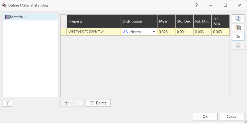
Define Material Statistics dialog - Distribution = Normal
- Mean = 0.026 MN/m3
- Std. Dev. = 0.001
- Rel. Min. = 0.003
- Rel. Max. = 0.003
- Click OK to close the Define Material Statistics dialog.
- Click OK again to close the Define Materials dialog.
3.2 Joint Property Statistics
To assign statistics to Joint Properties:
- Select Joints > Define Joint Properties
 . The Define Joint Properties dialog shows the mean parameter values for:
- Set 1 joint property:
- Strength Type = Mohr-Coulomb
- Cohesion = 0 MPa
- Phi = 30 degrees
- Override by Material = OFF
Waviness = 0 degrees.
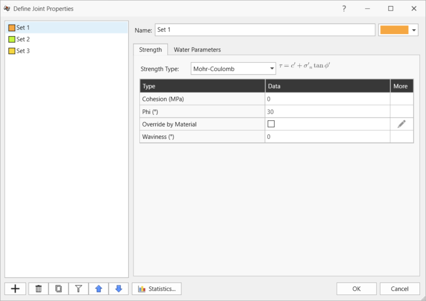
Deterministic values of Set 1 Strength joint property in Define Joint Properties dialog Water Pressure Method = Material Dependent. Water pressure computations on joints assigned with this joint property will depend on the Ru Value for Material 1.
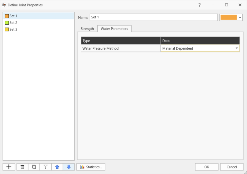
Deterministic values of Set 1 Water Parameters joint property in Define Joint Properties dialog
- Set 2 joint property:
- Strength Type = Mohr-Coulomb
- Cohesion = 0 MPa
- Phi = 35 degrees
- Override by Material = OFF
Waviness = 0 degrees.
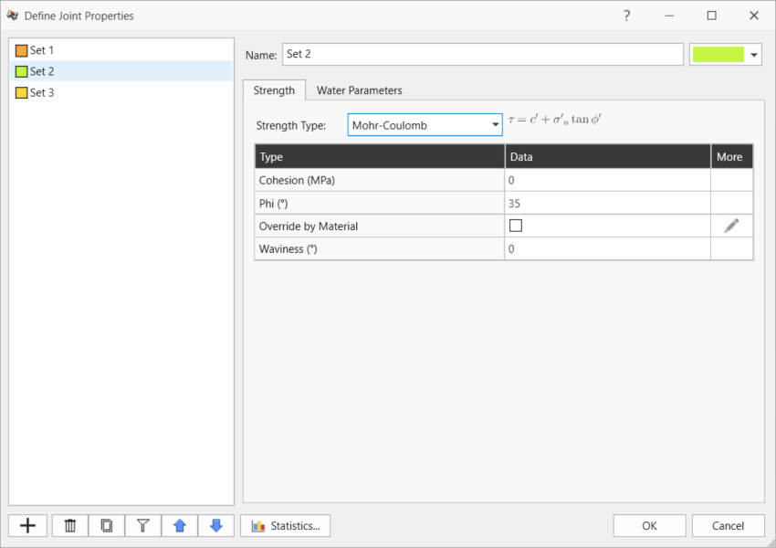
Deterministic values of Set 2 Strength joint property in Define Joint Properties dialog Water Pressure Method = Material Dependent. Water pressure computations on joints assigned with this joint property will depend on the Ru Value for Material 1. See the Groundwater Overview topic for more information about Ru Coefficient.
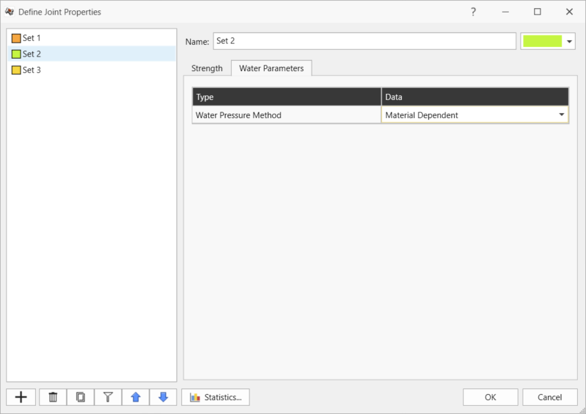
Deterministic values of Set 2 Water Parameters joint property in Define Joint Properties dialog
- Set 3 joint property:
- Strength Type = Mohr-Coulomb
- Cohesion = 0 MPa
- Phi = 15 degrees
- Override by Material = OFF
Waviness = 0 degrees.
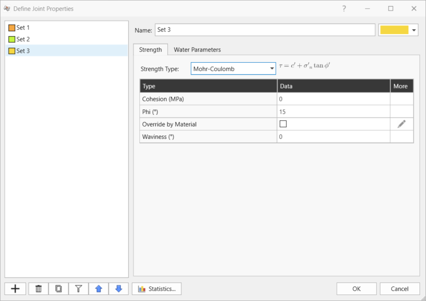
Deterministic values of Set 3 Strength joint property in Define Joint Properties dialog Water Pressure Method = Material Dependent. Water pressure computations on joints assigned with this joint property will depend on the Ru Value for Material 1.
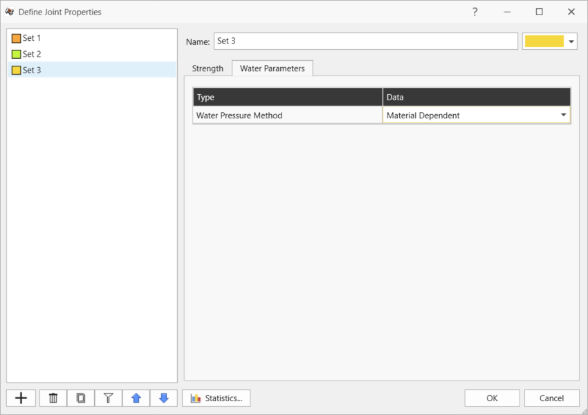
Deterministic values of Set 3 Water Parameters joint property in Define Joint Properties dialog
- Set 1 joint property:
Click the Statistics button.
The Define Joint Property Statistics dialog allows users to add any applicable inputs as random variables. There are three (3) Joint Properties.
The Define Joint Statistics dialog can also be accessed in Statistics > Define Joint Property Statistics- For the Set 1 joint property:
- Click the Add button.
- In the Add Random Variables dialog:
Select Phi.
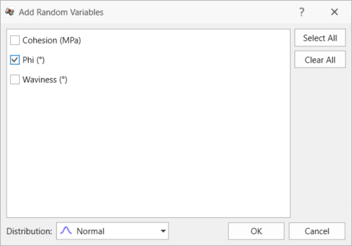
Add Random Variables dialog - Click OK. The Phi property is added to the grid with a Normal Distribution.
- Distribution = Normal
- Mean = 30
- Std. Dev. = 2
- Rel. Min. = 6
Rel. Max. = 6
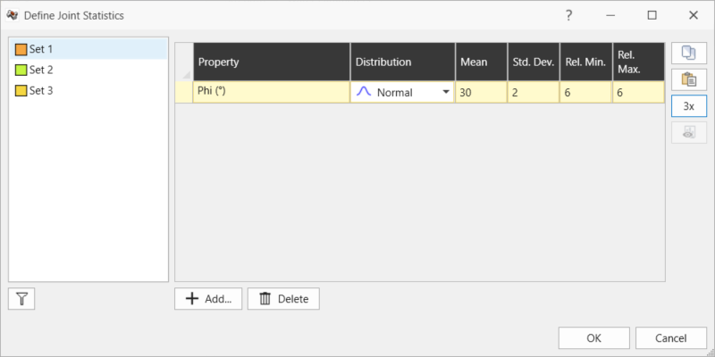
Set 1Joint Property statistics in Define Joint Property Statistics dialog
- For the Set 2 Joint Property:
- Click the Add button.
- In the Add Random Variables dialog:
Select Phi.
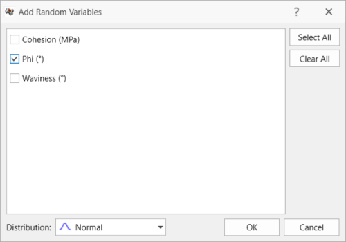
Add Random Variables dialog - Click OK. The Phi property is added to the grid with a Normal Distribution.
- Distribution = Normal
- Mean = 35
- Std. Dev. = 2
- Rel. Min. = 6
Rel. Max. = 6
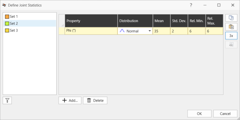
Set 2 Property statistics in Define Joint Property Statistics dialog
- For the Set 3 Joint Property:
- Click the Add button.
- In the Add Random Variables dialog:
Select Phi.
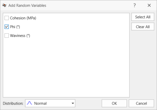
Add Random Variables dialog - Click OK. The Phi property is added to the grid with a Normal Distribution.
- Distribution = Normal
- Mean = 15
- Std. Dev. = 2
- Rel. Min. = 6
Rel. Max. = 6
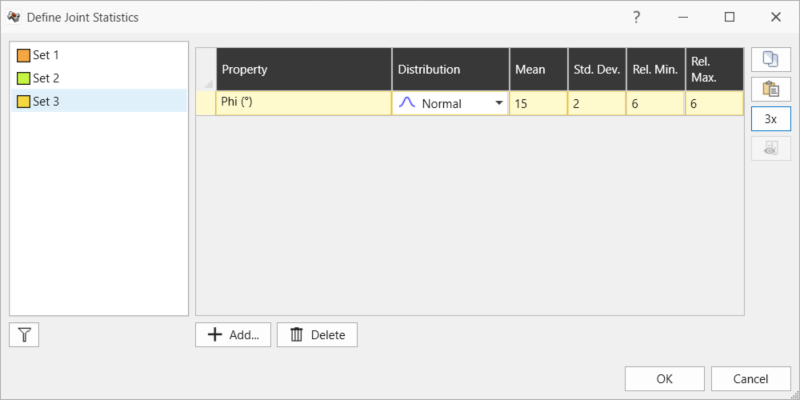
Set 3 Joint Property statistics in Define Joint Property Statistics dialog
- Click OK to close the Define Joint Statistics dialog.
- Click OK again to close the Define Joint Properties dialog.
4.0 Compute
RocTunnel3 has a two-part compute process.
4.1 Compute Blocks
The first step is to compute the unit blocks which may potentially be formed by the intersection of joints with other joints and the intersection of joints with the free surface.
To compute the unit blocks:
- Navigate to the Compute workflow tab

- Select Analysis > Compute Blocks

As compute is run, the progress bar reports the compute status. Once compute is finished, the Results node is added to the Visibility Tree and All Valid Unit Blocks are shown in the viewport. The Results node consists of the collection of valid unit blocks and the socketed excavation. The original External and Measured Joints visibility is turned off.
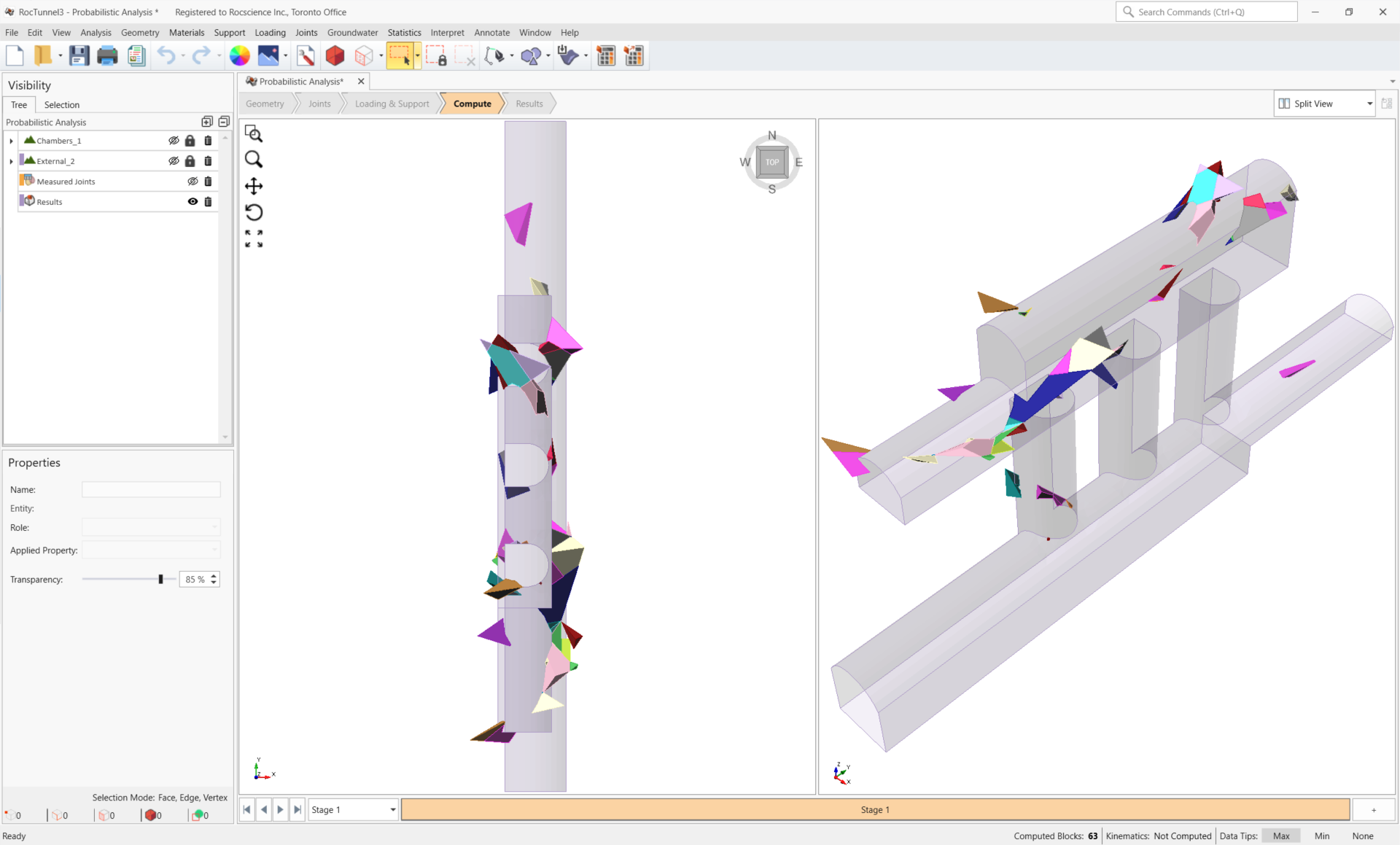
Once compute is finished, the unit blocks are colored according to the Block Color option (Random Colors) set in the Results node's Properties pane.
Compute Blocks only determines the geometry of the unit blocks. In order to obtain other information such as the factor of safety, Compute Kinematics needs to be run.
4.2 Compute Kinematics
The second and final compute step is to compute the removability, forces, and factor of safety for each of the valid unit blocks.
If Combined blocks is selected under Project Settings > Analysis, then this step also computes removable combined blocks and their factor of safety.
To compute the block kinematics:
- Ensure that the Compute workflow tab is the active workflow.
- Select Analysis > Compute Kinematics

- If the current Results Set is not already set to Removable Unit Blocks, then select the Results node from the Visibility Tree and set the Results Set = Removable Unit Blocks.
As compute is run, the progress bar reports the compute status. By default, after Compute Kinematics is run, only Removable Unit Blocks are shown.
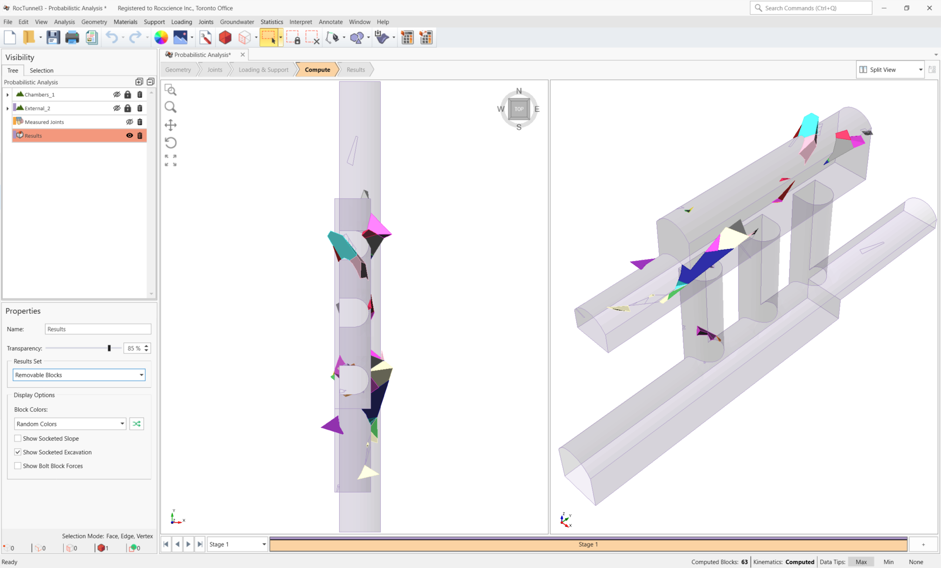
In this Probabilistic Analysis, for each unit block, the kinematics are computed 1,000 times, each time with statistically sampled inputs for Unit Weight of the Material 1 material property, and Phi for the Set 1, Set 2 and Set 3 joint properties, according to their respective random variables' distributions.
5.0 Interpreting Results
Since block geometry does not change between probabilistic runs (i.e., deterministic joint geometry), the visualization of the Results in the 3D CAD View is representative of all possible block geometries.
Once both blocks and kinematics are computed, all block results can be viewed in a grid format.
5.1 Block Information
To view all block results:
- Navigate to the Results workflow tab

- Select Interpret > Block Information

The Block Information pane shows the collection of blocks according to the Block Type and Results Set settings. The Block Type and Results Set shown can be selected in the Results tab of the Display Options, or the Properties pane for the Results node. In this case, only Removable Unit Blocks are colored and listed in Block Information.
In the case of a Probabilistic Analysis, for any given block, the Factors of Safety are affected by the random variables being sampled in each run. This then affects which blocks are considered "Failed" (i.e., Factor of Safety < Design Factor of Safety). In the case of Successive Removal, this also impacts the Removability of blocks which can only be removed if key blocks are removed. For these reasons, the definitions of the Results Set displayed are modified for a Probabilistic Analysis as follows:
- All Valid Unit Blocks: Identical as Deterministic Analysis since block formation is independent of the random variables for material and joint properties.
- Removable Unit Blocks or Removable Combined Blocks: For a given unit or combined block, if any sample run results in the block being Removable, then the block is included in the Results Set.
- Failed Unit Blocks (FS < Design FS) or Failed Combined Blocks (FS < Design FS): For a given unit or combined block, if any sample run results in the Factor of Safety < Design Factor of Safety, then the block is included in the Results Set.
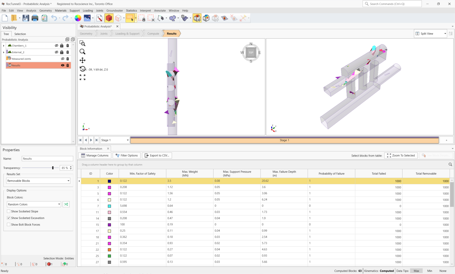
For Probabilistic Results, only the critical values among all sample runs are reported for each block:
- Minimum Factor of Safety
- Maximum Weight
- Maximum Required Support Pressure
- Maximum Failure Depth
- Probability of Failure
- Total Removable
- Total Failed
5.2 Contour Blocks
In RocTunnel3, blocks can be contoured by several metrics. In a Probabilistic Analysis, blocks can be contoured by any of the critical values.
To show block contours:
- Select Interpret > Contour Blocks

- From the Legend pane on the right, select Probability of Failure in the dropdown. The blocks are contoured by the Probability of Failure = Total Failed / Number of Samples.
- Any selected blocks are highlighted in PINK. To clear the selection for better visualization of contour colors, select Edit > Clear Selection (also available in the toolbar).
- Select Interpret > Zoom to All Blocks.
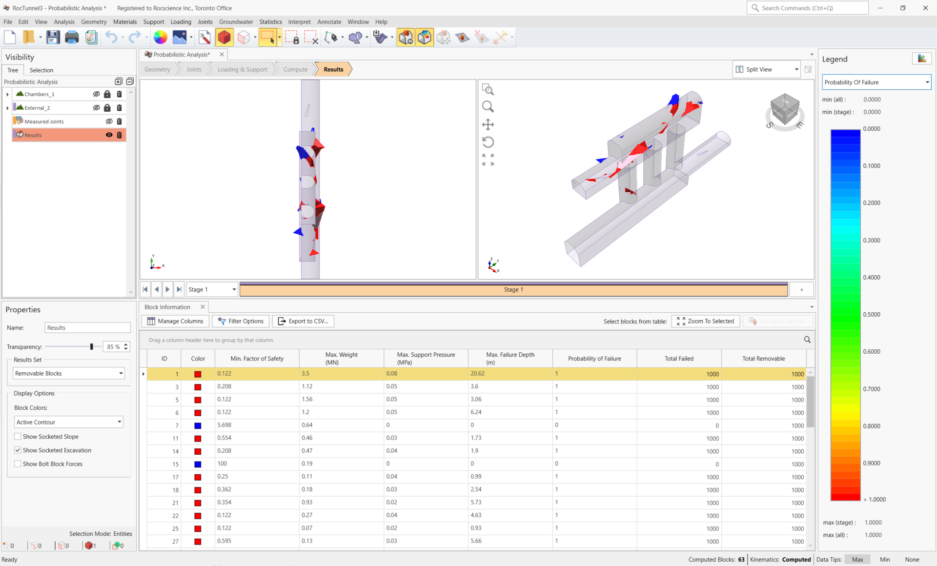
Note that probabilistic results, like deterministic results, are location-specific; where along the excavation and the shape of the blocks affect their stability.
6.0 Statistical Plots
Input or output distributions can be charted in the following forms:
- Histogram Plot
- Scatter Plot
- Cumulative Plot
Any random variables can be plotted in addition to computed block metrics such as Factor of Safety, Weight Required Support Pressure, Failed Depth, and Slope Face Area.
For each type of plot, the blocks considered in the plot data can be one of the three:
- Results Set (blocks considered in All Valid Unit Blocks, Removable Unit Blocks, Removable Combined Blocks, Failed Unit Blocks, or Failed Combined Blocks )
- Single Block (a single unit or combined block is considered, identified by Block ID)
- Filtered Blocks
6.1 Histogram Plot
Histogram Plots allow users to see the ordered frequency of a set of block data.
To plot a histogram plot:
- Select Statistics > Histogram Plot

- In the Histogram Plot dialog, enter the following:
- Data to Plot = Factor of Safety
- Number of Bins = 30
- Selection Method = Single Block
- Blocks to Plot = Single Block and Block ID = 1
- Select the Highlight Data checkbox and set the Factor of Safety < 1.5 to highlight any values less than the Design Factor of Safety.
- Select the Best Fit Distribution checkbox to plot the fitted distribution
Select Relative Frequency to scale the histogram Frequency axis such that the area under then distribution = 1. Otherwise, the Frequency is simply the count.
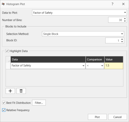
Histogram Plot dialog - Click Plot to generate the histogram.
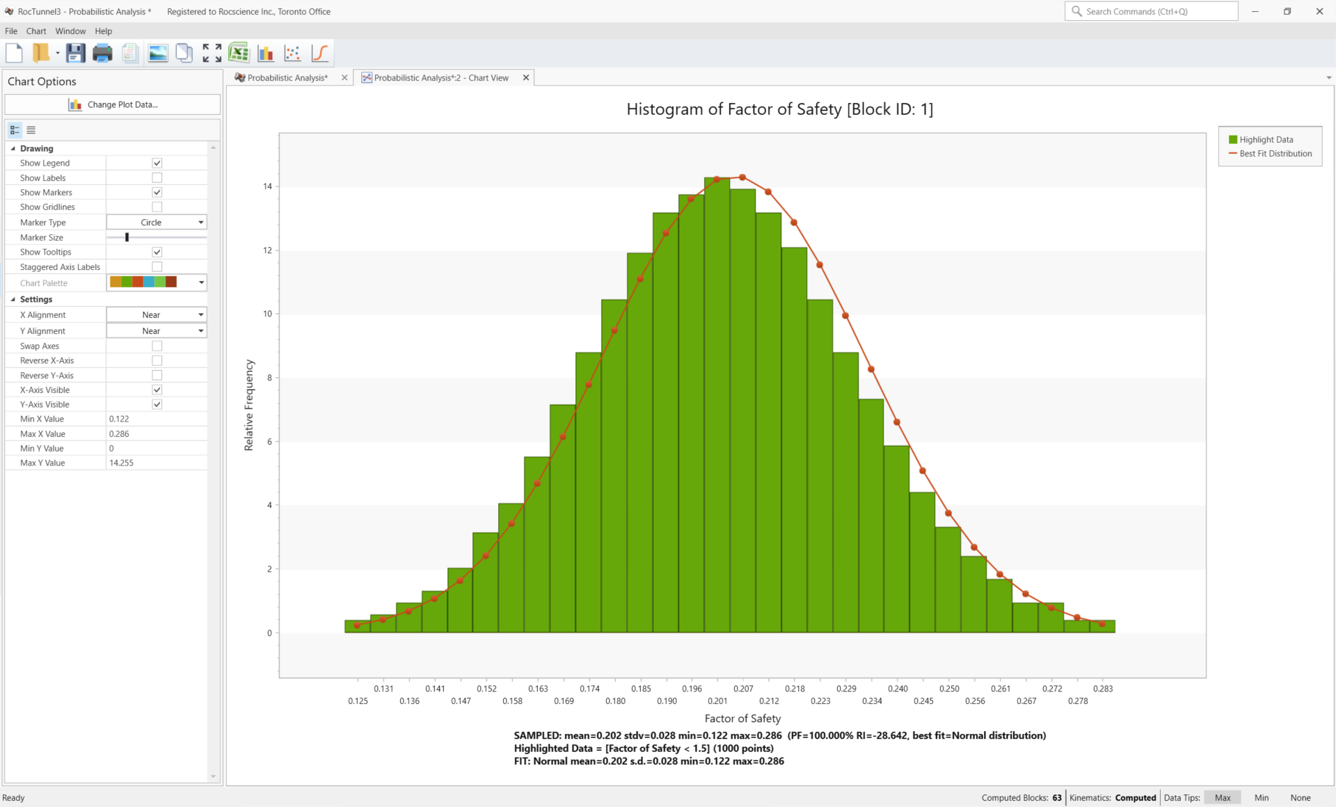
Relative Frequency is plotted on the y-axis, while Factor of Safety is plotted on the x-axis, lumped into 30 bins. The Best Fit Distribution shows the distribution type and parameters which best fit the data. The highlighted bars indicate the Relative Frequency of Factor of Safety < 1.5 (blocks which are kinetically unstable); all sample runs for this block results in a Factors of Safety < 1.5. The sampled mean, standard deviation, absolute minimum and maximum values are reported, along with the Probability of Failure (PF) and Reliability Index (RI) for the best-fit Normal distribution.
6.2 Scatter Plot
Scatter Plots allow users to see the correlation between two sets of block data.
To plot a scatter plot:
- Navigate back to the 3D Geometry View by selecting the tab below the toolbar at the top of the screen.
- Select Statistics > Scatter Plot

- In the Scatter Plot dialog, enter the following:
- Horizontal Axis = Factor of Safety
- Vertical Axis = Set 1: Phi
- Selection Method = Single Block and Block ID = 1
- Select the Highlight Data checkbox and set the Factor of Safety < 1.5 to highlight any values less than the Design Factor of Safety.
Select the Regression Line checkbox to plot the line of best fit.
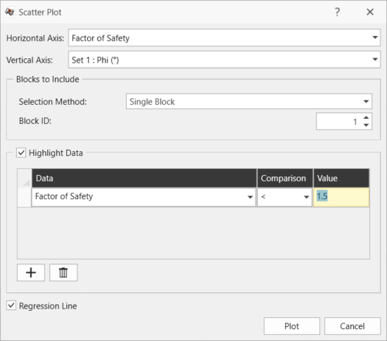
Scatter Plot dialog - Click Plot to generate the scatter plot.
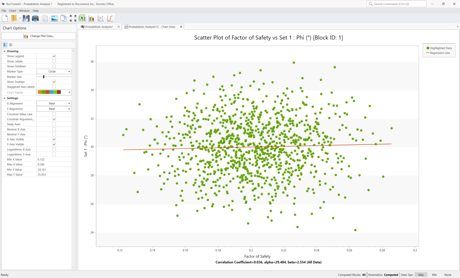
The Regression Line and tight clustering of the scatter plot data points around that line indicates that there is a strong correlation between Factor of Safety and Friction Angle of the Set 1 joint property.
6.3 Cumulative Plot
Cumulative Plots allow users to see the cumulative probability of a set of block data.
To plot a cumulative plot:
- Navigate back to the 3D Geometry View by selecting the tab below the toolbar at the top of the screen.
- Select Statistics > Cumulative Plot

- In the Cumulative Plot dialog, enter the following:
- Data to Plot = Weight
- Number of Bins = 30
- Selection Method = Results Set
- Results Set = Failed Unit Blocks
Stage to Use = Stage 1
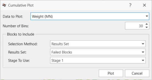
Cumulative Plot dialog - Click Plot to generate the cumulative plot.
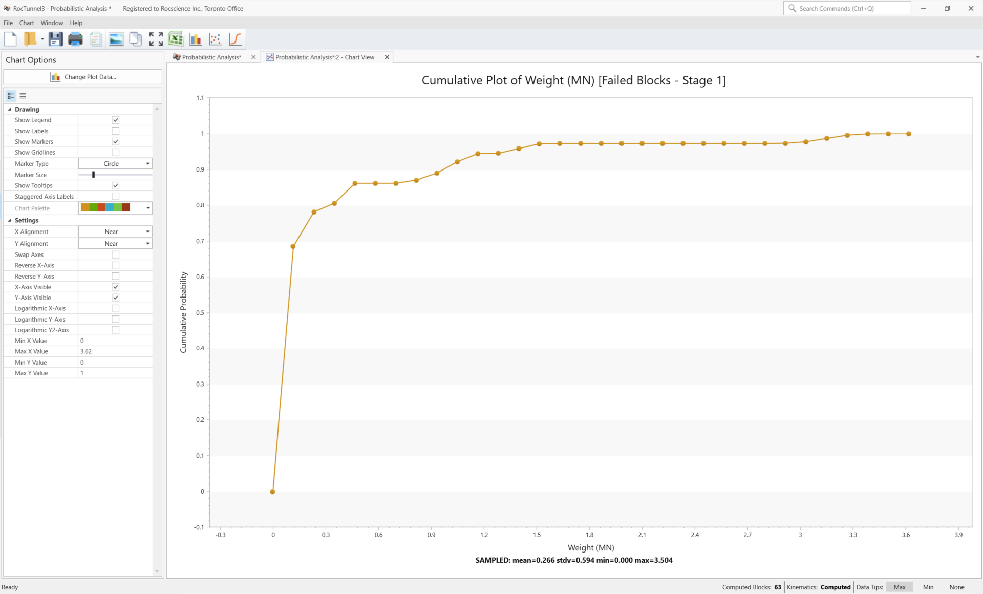
The cumulative plot shows the cumulative distribution of block Weight values for the Failed Unit Blocks Results Set. At any given Weight value, the Cumulative Probability is the percentile (as a fraction) of unit blocks sampled which have a Weight less than or equal to that value. Similarly, looking at some percentile we can get the corresponding Weight value (e.g., 90th percentile would correspond to approx. Weight = 1 MN).
Additional Exercise
To see the relationship between the Relative Frequency of block Weight, plot a histogram of Weight:
- Select Statistics > Histogram Plot
- In the Histogram Plot dialog:
- Set Data to Plot = Weight
- Set Number of Bins = 30
- Set Selection Method = Results Set
- Set Results Set = Failed Unit Blocks
- Set Stage To Use = Stage 1
Select Relative Frequency to scale the histogram Frequency axis such that the area under then distribution = 1.
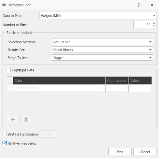
Histogram Plot dialog - Click Plot to generate the histogram.
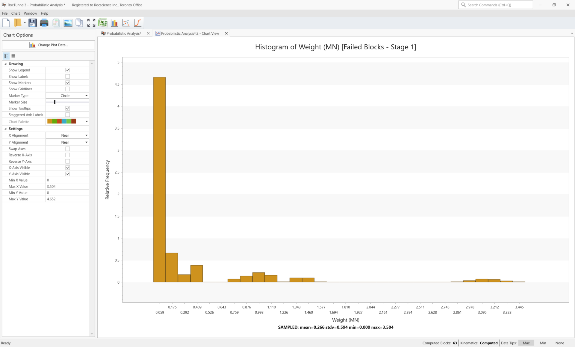
The Weight Cumulative Plot from Section 6.3 is essentially the cumulative sum of the Relative Frequency of Weight in the Histogram Plot.
This concludes Tutorial 4.