Spatial Safety Maps from RS3 SSR Results: A Python Post-Processing Workflow

Introduction

Shear Strength Reduction (SSR) analysis is a well-established method for assessing the stability of slopes and other geotechnical infrastructure, including open pits. In RS3, SSR yields a single critical Strength Reduction Factor (SRF) for a model (which is equivalent to the factor of safety). This is the highest reduction factor at which the modelled system remains stable; any small increase in this factor causes the model to be unstable. Although the number is essential for design, it does not by itself show where secondary failure modes or other local mechanisms develop.

Limit equilibrium tools such as Slide3 address this through surface safety maps – contours of local factor of safety superimposed on the topography or slope surface, revealing multiple candidate mechanisms rather than only the global minimum. A similar idea has been demonstrated in distinct-element and continuum software, where kinematic failure indicators, such as gridpoint velocity, are produced at each trial factor of safety during an SSR search and used to contour the highest factor at which each location remains stable. This article describes a workflow that extends the idea to standard RS3 SSR analysis and to developing a spatial safety map.

A Python post-processing script reads nodal displacements for all computed SRF stages, applies a user-defined displacement threshold as a local failure criterion, and contours the points that attain the threshold. 

Shear Strength Reduction in RS3 

In SSR, material strength parameters are scaled by a factor F (the SRF) while elastic stiffness is held constant. The analysis searches for the critical value of F at which the model is no longer stable. 

Mohr–Coulomb (MC)

For Mohr–Coulomb materials, the strength factor reduces cohesion and friction as follows: 

c′ = c / F ,     φ′ = tan-1( tan φ / F ) 

Tensile strength, if used, is typically scaled in the same manner. The analysis proceeds by solving successive equilibrium problems at increasing F until a non-convergent (or otherwise unstable) state is identified. The critical SRF is the factor associated with that onset of global instability. 

Generalized Hoek–Brown (GHB) 

For Generalized Hoek–Brown materials, the equivalent approach is to reduce the shear strength envelope consistently with the selected SRF. This is done by dividing the GHB failure function by the factor F and then determining a new set of GHB parameters that fit this lowered envelope. As with the Mohr–Coulomb framework, the elastic modulus is not reduced; only the strength is scaled so that the critical SRF retains the interpretation of a global factor of safety against shear failure.

Constructing a Safety Map from SSR Results with Python Scripting 

The global critical SRF answers: At what factor does the system fail? The safety map answers a complementary question: At what factor does each location first show a signature of failure? 

The post-processing workflow is as follows: 

1. Run SSR in RS3 to obtain the critical SRF and a sequence of result states at all trial (or sampled) SRF values. 
2. Export nodal results for every available SRF—displacements at all nodes in the mesh. 
3. Define a displacement threshold u_lim (user input). A node is treated as having “failed” at a given SRF when its displacement magnitude first meets or exceeds u_lim. 
4. Assign a local SRF to each node: the lowest SRF at which that displacement criterion is satisfied. Nodes that never reach the threshold within the computed range are assigned a high (or capped) value for plotting. 
5. Contour the local SRF field on the excavation/ground surface and on user-selected cutting planes. 

The contours are generated by a Python viewer that connects to RS3 Interpret through the scripting API and reads results from the computed model. It first reads the list of stored SSR trials, then, for each trial, requests the solid mesh from Interpret and streams the nodal displacement field. Element connectivity is taken once from the same mesh (the nodes attached to each element). Coordinates, connectivity, and the per-node displacement history are cached locally. From that volume mesh, the viewer extracts the exterior triangular faces and colour-maps them as a 3-D surface; a cutting-plane view is formed by intersecting element edges with a user-chosen plane and interpolating nodal values onto the cut.

The resulting contour is a spatial safety map: warm colours mark regions that mobilize at or near the global critical SRF; cooler colours mark regions that only reach the displacement criterion at higher factors or not at all within the bracketed range. 

Case Study: Open-Pit Mine

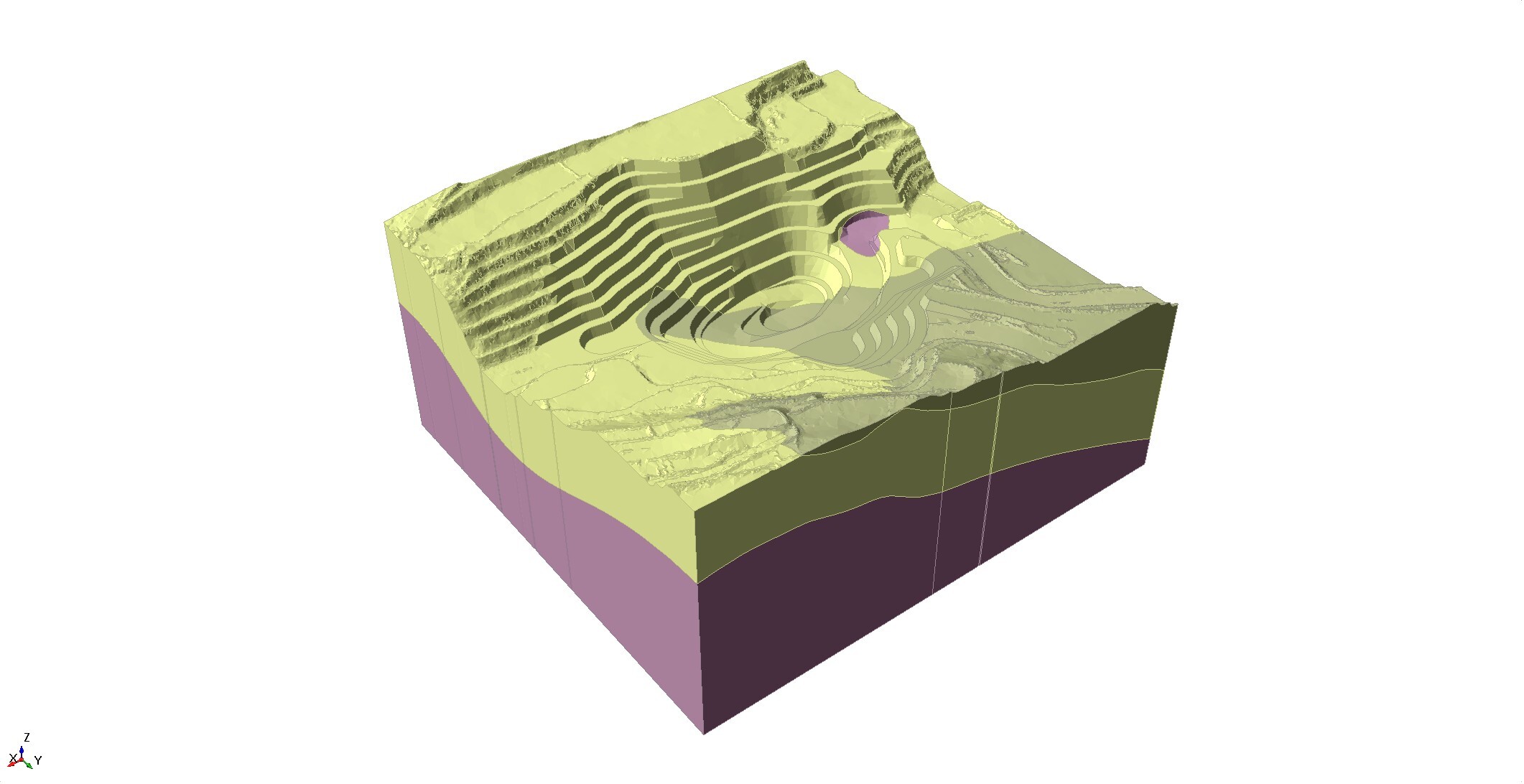
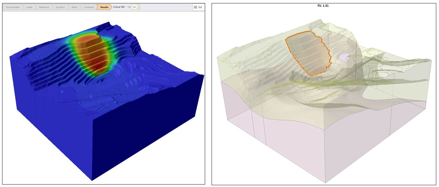
The method was tested on a large open-pit model, with the lithology and bench geometry shown in Figure 1.  The Mohr–Coulomb material model was used to describe the behaviour of the mine’s three main materials. The finite-element mesh comprised approximately 500,000 higher-order tetrahedral elements.

SSR analysis was performed in RS3, and the critical SRF of 1.3 was calculated. An equivalent Slide3 limit-equilibrium analysis gave a minimum factor of safety of 1.31, providing strong agreement on the global stability number. 

The Python safety-map script was then applied using a user-defined displacement threshold. Contours of local SRF on the pit surface (Figure 3) show that the lowest values are concentrated along the steep benches of the pit — consistent with the expected critical mechanism — while peripheral topography remains much more stable.

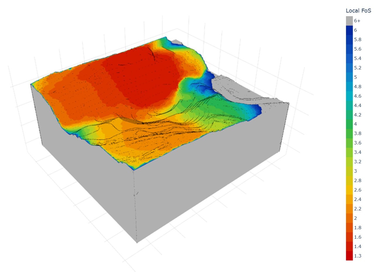
For the same geometry, Slide3 identifies a discrete critical slip mass on the stepped pit wall (Figure 2)—outlined on the benches where the LEM search finds the global minimum (FS ≈ 1.31). That mechanism coincides with the warmest (lowest-SRF) region of the RS3 safety map in Figure 3, linking the continuum displacement-threshold contours to the LEM critical failure surface. 

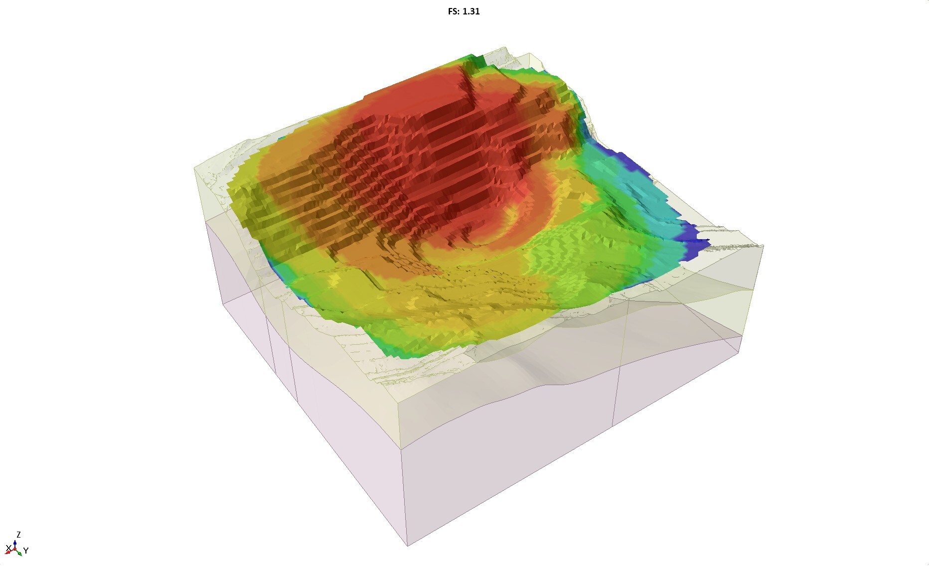
Slide3’s surface safety map (Figure 4) extends that single-surface result into a spatial ranking of local factors of safety. The pattern of low-FS zones along the pit walls, and higher-FS regions away from the walls, closely compares to the RS3 map. Locations that remain stable to higher SRFs in the displacement-based FE map align with higher local factors of safety in the LEM safety map.

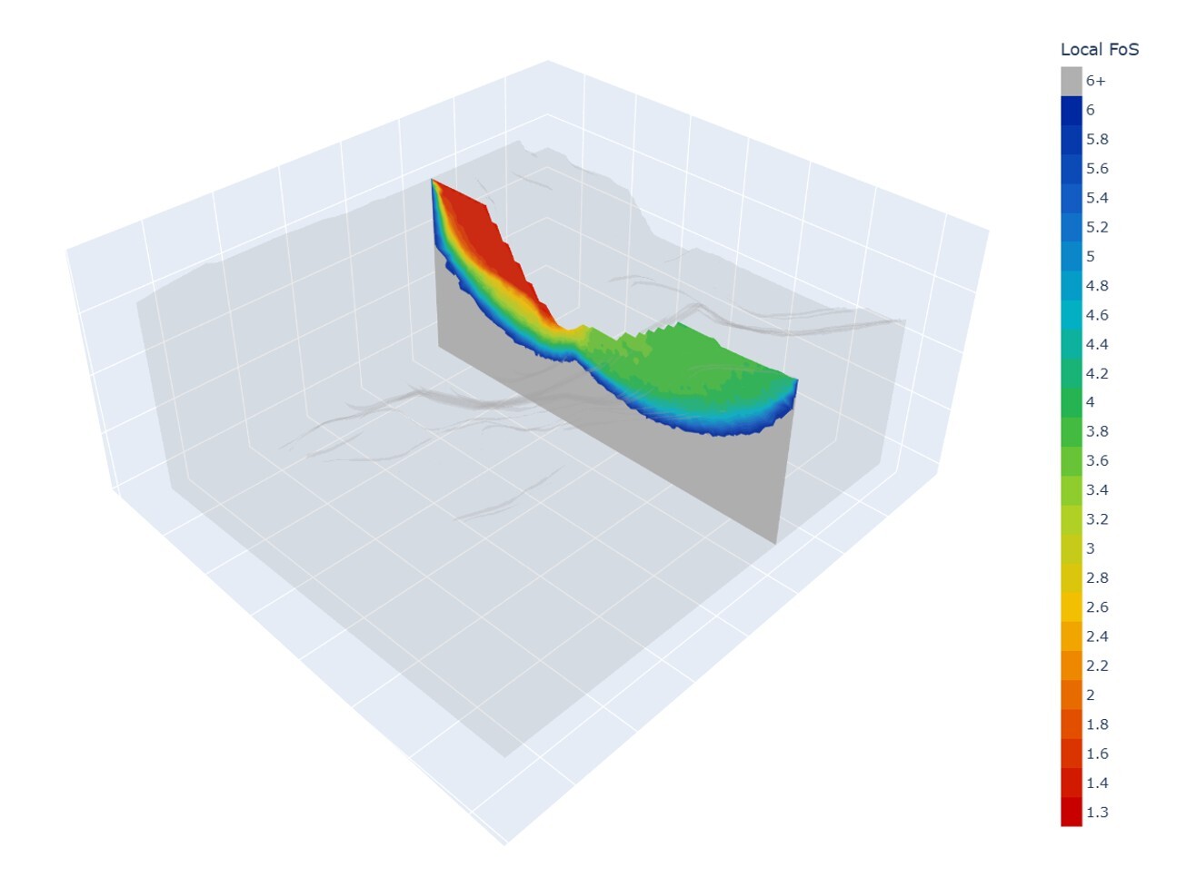
Beyond the free surface, the script can display the same local-SRF field on cutting planes through the mesh, allowing inspection of the depth and shape of mobilizing zones in cross-section—information that is particularly useful for multi-bench and bermed profiles where more than one mechanism may be present. 

Comparison with Limit Equilibrium Safety Maps 

Agreement between the RS3 safety map and Slide3 in this example is encouraging, but it should not be expected in every case. 

• SSR displacement safety maps inherit the full continuum solution: displacement magnitude depends on constitutive model, flow rules, elastic stiffness, boundary conditions, and the chosen threshold u_lim.

Consequently, two models with identical strength parameters but different moduli (or different threshold choices) can produce different spatial maps even when the global critical SRF remains similar. Tuning of the displacement cutoff, which is analogous to selecting a velocity limit in other SSR contouring methods, forms part of engineering interpretation; it is not a purely automatic constant. 

Used together, these views are complementary: Slide3 provides both the critical mechanism (Figure 2-b) and a strength-based spatial ranking of surfaces (Figure 4); RS3 SSR provides the global critical SRF from continuum mechanics; and the displacement-based safety map (Figure 3) extends that SSR sequence into a spatial picture of progressive mobilization.

Conclusions 

RS3 already delivers a robust critical SRF through shear strength reduction. Its new Python scripting capabilities allow results to be post-processed in any desired way, such as creating spatial safety maps from RS3 SSR analysis. The method offers a practical route—within the existing RS3 SSR framework — to visualize multiple mobilizing regions in complex 3D excavations, on model surfaces and along cutting planes. It remains transparent about the role of stiffness and threshold selection when compared against pure strength-based LEM maps.