Introduction

This article depicts how the pile analysis under lateral loading, or couples is improved in RSPile by updating the pile flexural stiffness during the solution in cases of piles with combined flexural and axial stresses. This is raised because of the bending (flexural) stiffness of the pile varies with the level of cracking and the applied axial load. In previous versions and in most of software the bending stiffness-moment relation is a single curve constructed in the beginning of the analysis and never updated or varied along the pile length. Usually, that curve is based on the loading of the pile head while pile load may change at other depths as well, which may have significant effect on the flexural stiffness.

In the latest version of RSPile release 3.014, this issue is addressed and solved. The results of the pile analysis with updated bending stiffness clearly varies with depth during the analysis. An example is solved in this article to compare the results between single and variable moment-curvature curves (bending stiffness) with depth.

Theoretical background

In piles with reinforced concrete sections, one of the parameters for the analysis of piles under lateral loading or bending moments is the bending (flexural) stiffness, effective EI. In ACI 318–2019, and similar codes around the world, the effective EI may be approximated by the concrete modulus of elasticity, E_c , multiplied by an effective moment of inertia Ie , a value falling between the cracked section moment of inertia, I_cr , and the gross moment of inertia, I_g. Most of the pile analysis methods depend on a constant bending stiffness throughout the analysis. For LRFD analysis half of the gross moment of inertia will be acceptable and for the serviceability levels a gross moment of inertia may be an adequate value to use. With the spread of computer software for pile analysis, the bending stiffness is not constant anymore in the analysis and better value for EI is estimated during the iterations of the solution of the beam-column differential equation (by FEM or FDM methods) relating it to the last calculated curvature of the beam at that step of iteration φ_i where i refers to the iteration. The easiest method to calculate an updated bending stiffness for a specific point at the beam in an iteration step, (EI)_i , is the relation,

(EI)_i= M_i/φ_i

Derivation for this relation may be found in classical textbooks of strength of materials, see for example Higdon et al. (1978). The moment curvature curve is prepared from the beginning to pick the corresponding EI at any moment-curvature level. This helps getting better results for the response of the pile to the applied loads.

The bending stiffness is highly dependent on the applied axial load at the section and the axial load varies with depth due to the soil resistance around the pile, i.e., the skin friction. The skin friction decreases the axial load with depth (or increases it in the case of negative skin friction) and it may also vary due to additional external loads applied on the pile at different depths.

In traditional pile analysis the bending stiffness is taken constant along the depth which is true for elastic sections. Engineers in hand calculations or simple spread sheets assume the reinforced concrete pile as an elastic section. Meanwhile, most of the software programs the relation between bending stiffness and the bending moment in reinforced concrete sections is assumed unchanged and a single M-φ curve is used for the whole length of the pile (just like a column in a structural frame). Reese and Van Impe (2011) stated that “the errors that are involved in using the approximation where there is a change in the bending stiffness along the length of a pile are thought to be small but must be investigated as necessary”. Nevertheless, the error increases with new external loads added to the pile through the depth and in several other cases such as changes in section dimensions or materials (e.g. reinforcement ratio). This error is overcome in the recent version of RSPile 3.014.

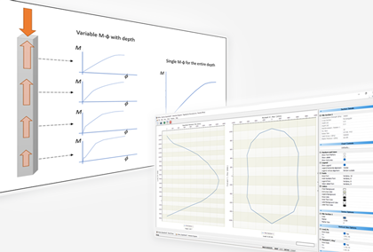
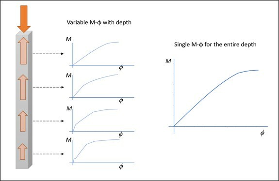
This is accomplished by generating a series of moment-curvature curves based on the range of internal axial force experienced by the pile. The bending stiffness of the reinforced concrete pile is then obtained as a function of both internal axial force and curvature. Fig.1 depicts the difference between the use of a single M-φ relation and multiple ones in the modeling.

Example problem

Pile section and soil model

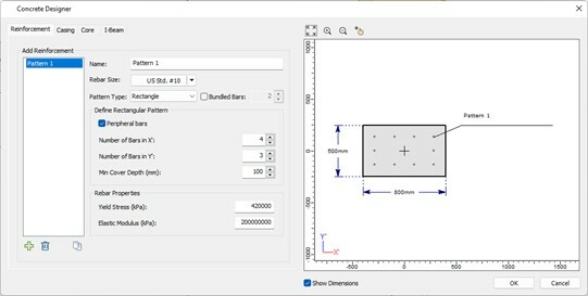
A pile with a rectangular reinforced concrete section of 500 mm depth and 800 mm width with 34 MPa concrete strength and reinforced with 10 #10 bars placed peripherally at 100mm cover. The pile is analyzed using RSPile under a lateral load in the long side direction of 150 kN applied at the pile head investigating the response applying different vertical downward loads at the top of the pile, 100 kN, 500 kN and 1000 kN. The section details are shown in the section designer of RSPile in Fig.2.

Pile length is taken as 20 m fully embedded in soil. To control soil parameters effects, the soil is assumed elastic with a constant modulus of lateral subgrade reaction of 1000 kN/m³ and a skin frictional spring of 10000 kN/m³ while the end bearing stiffness is set to zero to govern the axial load distribution by the skin friction only.

Section structural capacity

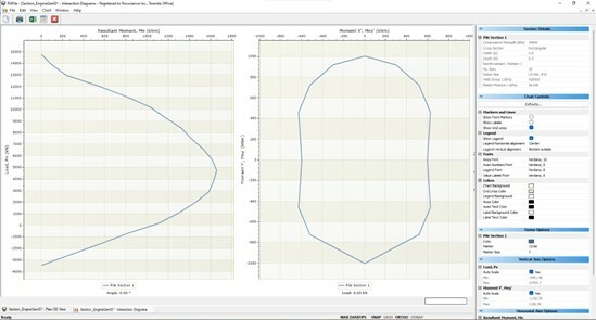
With the introduction of Interaction Diagrams in RSPile, users can now estimate the structural capacity of their concrete section in a single click. Fig.3 shows interaction diagram for the short column (pile), the nominal axial load capacity, P_n plotted against the nominal bending moment capacity M_n for a load applied at an angle α of 0^o taken counterclockwise from x’ axis. At the right side the M_nx’-M_ny’ plot is presented for a case of P_n=0 though the user may choose any load level within the pile capacity. From the left graph the three axial loads 100 kN, 500 kN and 1000 kN chosen for the example can be found being safe enough with the correspond moments that will be obtained in the analysis part.

Effects of a vertical load on pile response

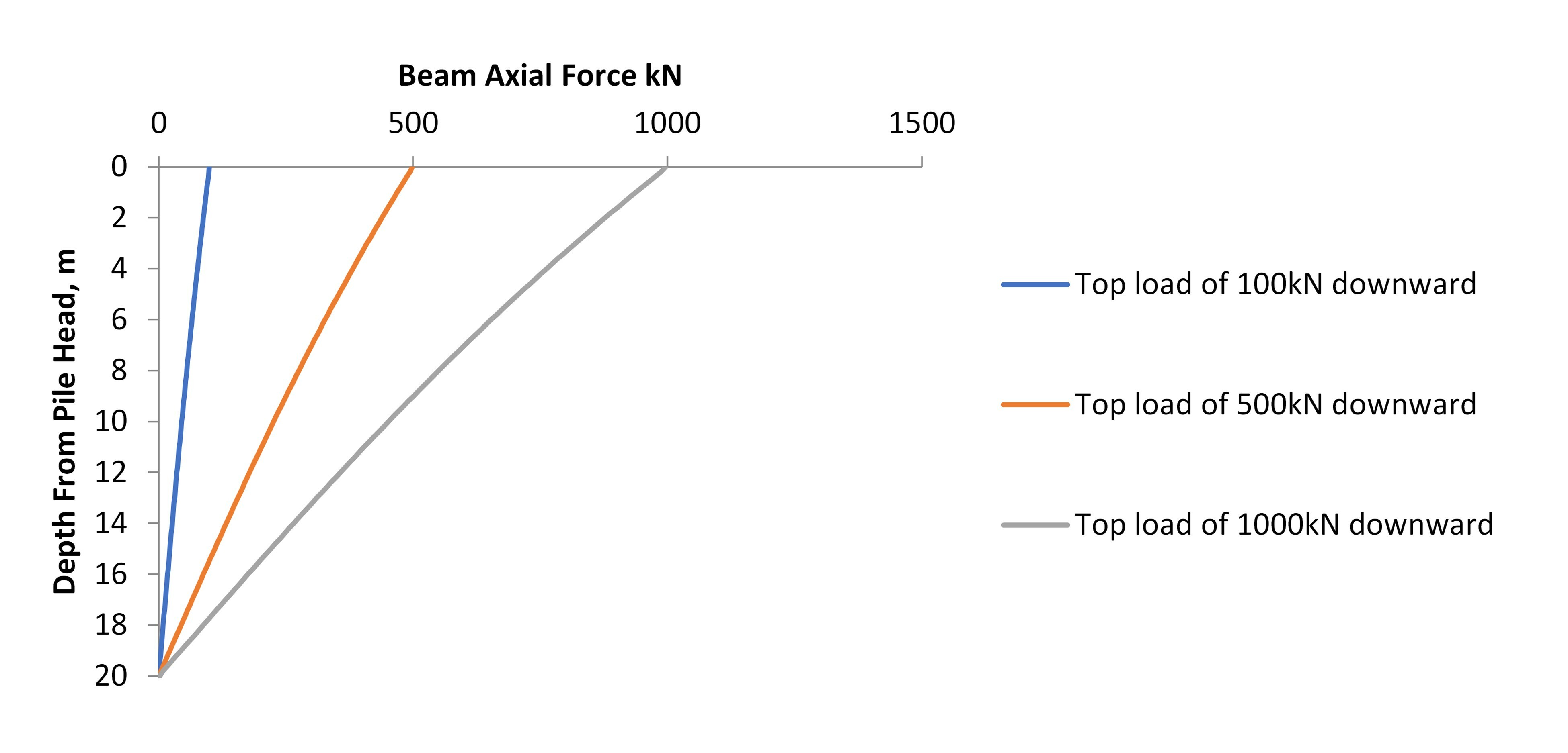
Fig.4 shows the distribution of axial force through the depth which should be varying from the load applied at the pile head to zero at the bottom as no force is transferred to base (resistance is side resistance only). The model is run with RSPile v.3.013 (single M-φ curve) and with the improved bending stiffness calculations with varying M-φ curves updated for each depth based on the axial force remaining at that level which is included in RSPile v3.014.

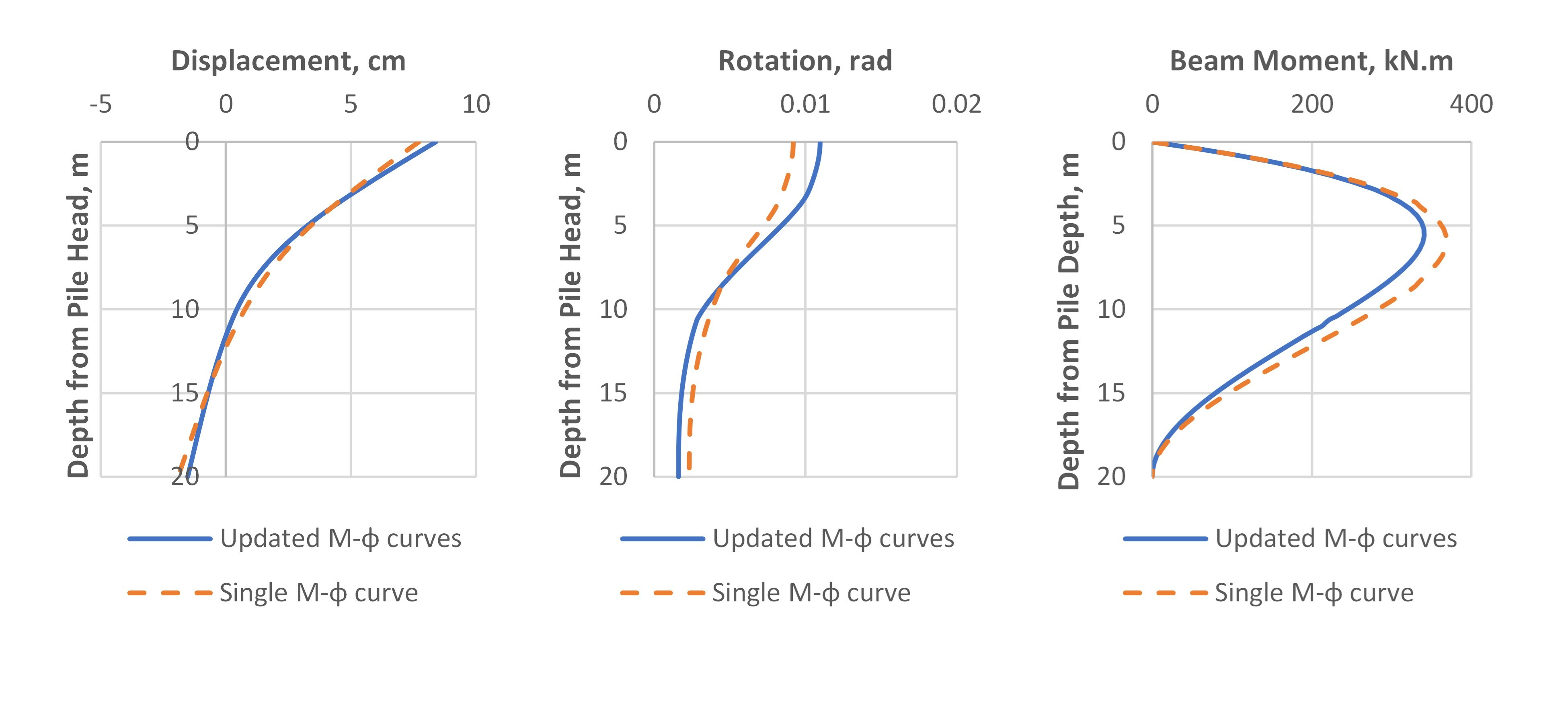
The results for calculated lateral displacements, rotations and calculated bending moment are plotted against depth for both solutions in Fig.5, Fig.6 and Fig.7 for applied downward vertical loads of 100 kN, 500 kN and 1000 kN respectively.

The differences between the results using a single M-φ curve for the entire length of the pile and the results in the case of enhanced bending stiffness updated with M-φ curve for the axial load at the level of the beam element can be detected easily. The single M-φ is constructed for the section of the pile with an axial load equal to the applied load at the top.

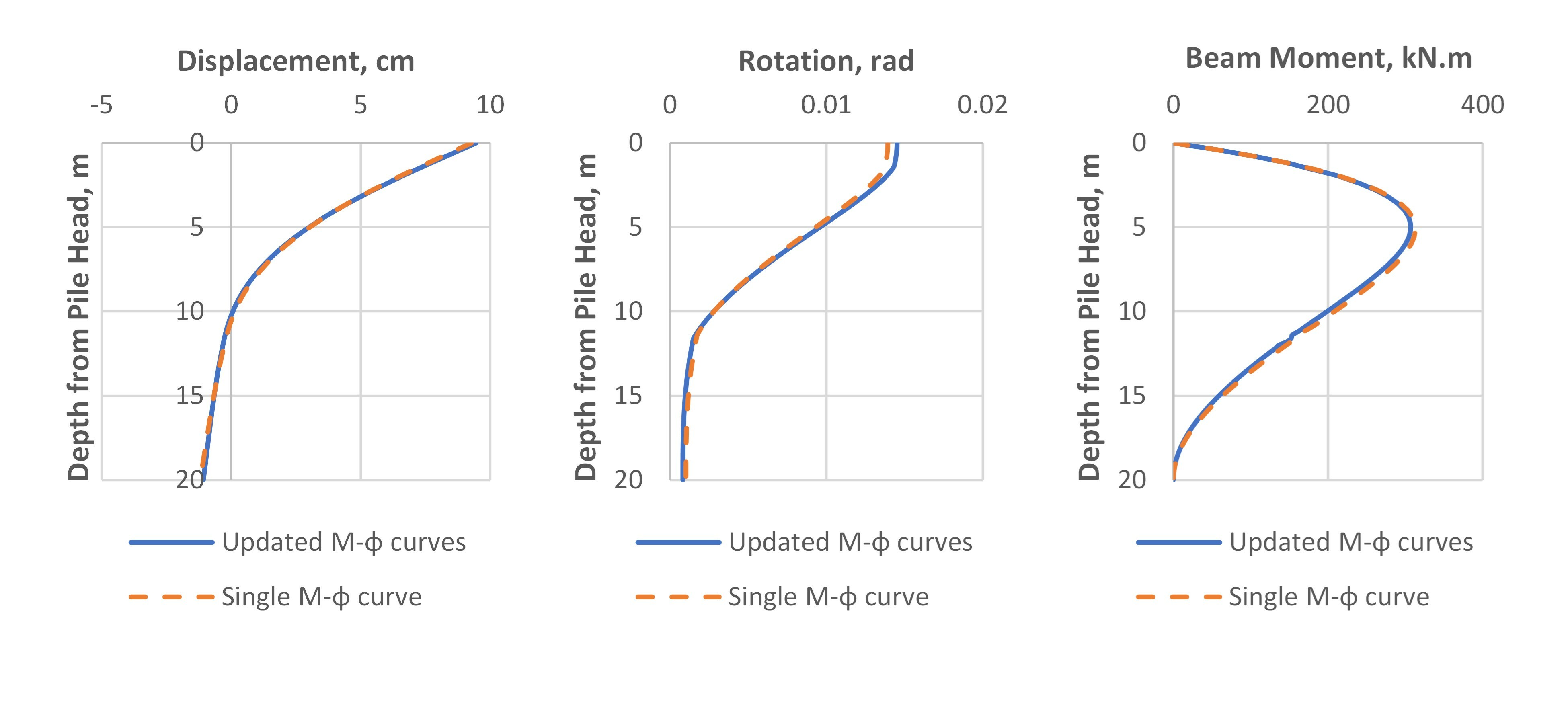
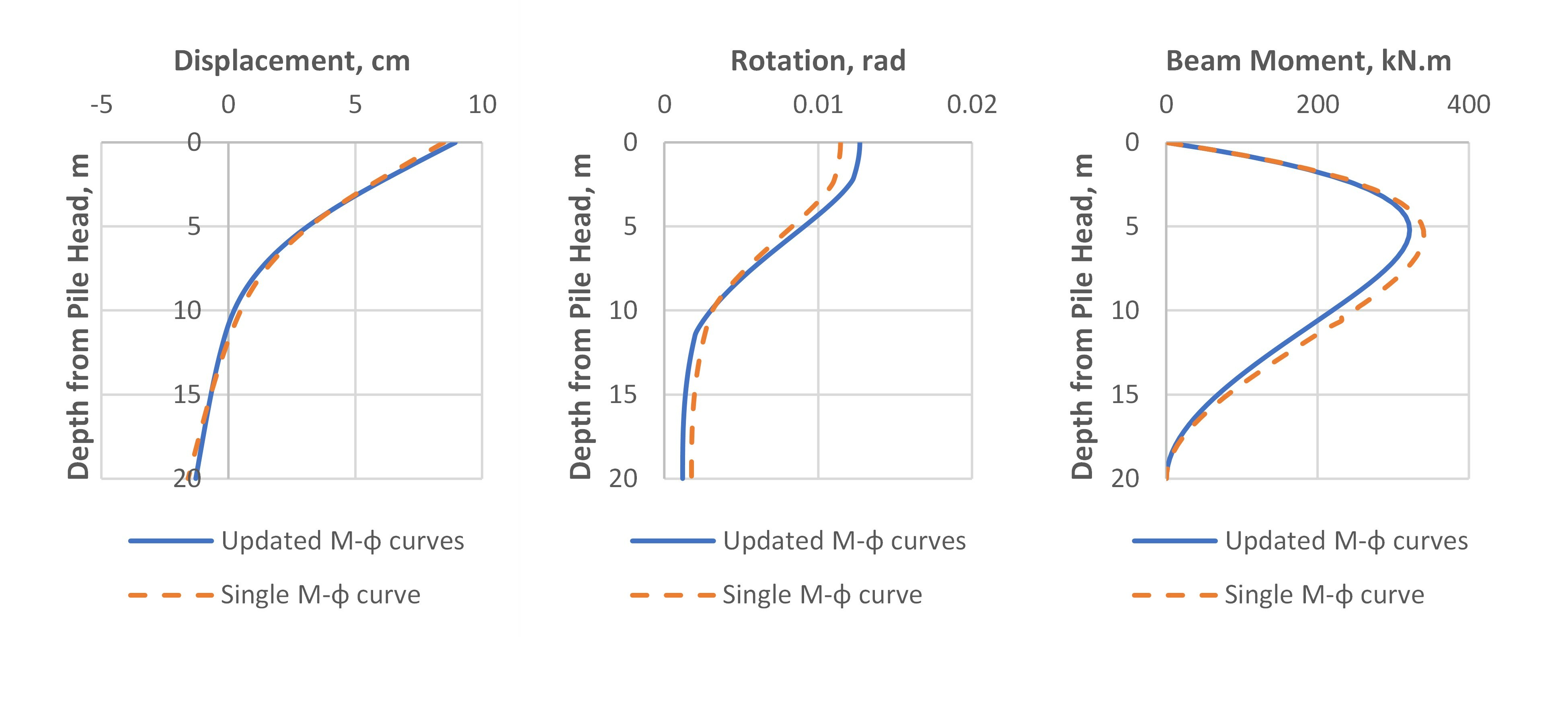
Discussion

As it is expected, the variation in the results between the case with single M-φ curve and the case with multiple M-φ curves would be insignificant if the applied external axial load is small so when the load is 100 kN there is not much difference in displacement or other output. Things get different when the load is increased. It could be clearly seen how the differences increased between single M-φ curve application and the improved analysis case with varying M-φ curves through the depth under 500 kN and 1000 kN. It should be noted that if there is no soil resistance at the pile skin the axial force in the section will not change and the bending stiffness will follow the same M-φ curve. As the axial compression force decreases with depth due to soil skin resistance, the bending stiffness decreases as well and if the moments will remain almost at the same level (the bending moment gets affected with the variation of bending stiffness but in less percentage) the deflection and the rotation will increase. The pile response to applied lateral loads will be higher at the pile parts closer to the load and the bending moments calculated will be more than if a single M-φ curve is applied.

The above finding means that the original single M-φ curve usage for the entire length of the pile is less conservative, and the estimated displacements and rotations are lower. An opposite behavior is expected when an upward load is applied at the pile head (i.e. tensile axial forces are developed inside the pile elements) as the bending stiffness increases while consuming the tensile force by the skin resistance through the depth.

Conclusion

The new improved bending stiffness calculations using updated M-φ curves through the pile depth is better to follow and the results are supposed to be more accurate. Whether under tension or compression the pile response intensity will get closer to the applied load rather than distributed along farther portions. Further investigation may be done to find out the effects of updating the bending stiffness with different points of load application, traction loads, and different load directions with RSPile 3.013 version or other commercial programs which that uses single M-φ curve and the 3.014 release of RSPile.

References

Higdon, A., Ohlsen, E., Stiles, W.B., Weese, J.A. and Riley, W.F. (1978): “Mechanics of Materials”. SI version, 3^rd ed., John Wiley and Sons, New York, USA, 752pp.

Reese, L.C. and Van Impe, W. (2011): “Single Piles and Pile Groups Under Lateral Loading”. 2^nd ed. Taylor & Francis Group LLC, Boca Raton, USA.

More from Rocscience