3D Limit Equilibrium Method (LEM): A Parallel Case Study of a Landslide Supported with Piles
Shedding light on the preventative measures against slope failure due to stresses
Determining the accuracy of slope stability analysis has been a primary subject of interest in the geotechnical field for several decades now. Taking preventative measures against slope failure is crucial to minimize casualties and damage to infrastructure. The limit equilibrium method (LEM) and finite element method (FEM) are the two most reliable approaches used by researchers and engineers.
This study provides insights into a 3D Limit Equilibrium analysis of a landslide model supported with piles. It considers the capacity of the pile as being constant or non-linear; the latter of which is determined using a separate Finite Element (FE) software for pile analysis.
Summary of the Model
Soil profile
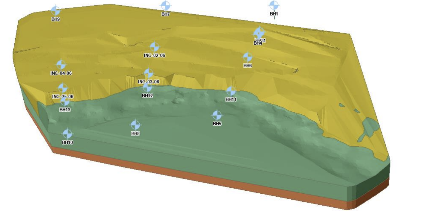
LEM model: existing soil layers and material properties are detailed in Table 1.
Material Name |
Unit weight (lbs/ft3 ) |
Strength Type |
Cohesion (psf) |
Phi (deg) |
API Sand |
125 |
Mohr-Coulomb |
0 |
35 |
Sand |
112 |
Mohr-Coulomb |
0 |
15 |
Sand Reese |
142 |
Mohr-Coulomb |
0 |
40 |
Table 1. Existing soil properties for the model
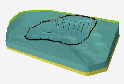
To simulate the LEM analysis assumptions, the Janbu and Spencer methods were adopted. Fig 1. shows multiple boreholes that were used to construct the material boundaries.
Nonlinear Capacity Piles
Soil parameters for the pile analysis are outlined in Table 2.
Model |
Unit weight (Ibs/ft3) |
Friction Angle (deg) |
Initial Modulus of Subgrade Reaction |
Strain Factor |
Undrained Shear Strength |
API Sand |
125 |
34 |
140 pci |
- |
- |
Sand (Reese) |
112 |
15 |
10 pci |
- |
- |
Sand |
142 |
40 |
200 pci |
- |
- |
Analysis results and discussion
Unreinforced slope model
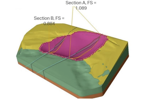
The analysis results of the unsupported slope using LEM have been shown in Fig. 2. The experiment has identified a critical slip surface with Spencer FS = 1.17. Sections A & B were created within the 3D model to analyze the 2D results shown in the right of Fig. 2.
Note that the FS in 2D is generally lower than the 3D FS (Stark and Ruffing 2017).
Analysis of the Nonlinear Capacity Pile
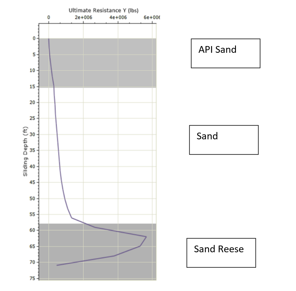
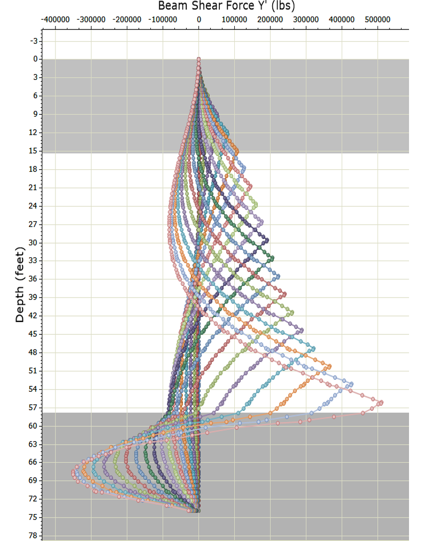
The analysis of piles was carried out using RSPile software which conducts Finite Element analysis to examine the nonlinear capacity of piles. In this case, RSPile is used to generate the lateral resistance envelope corresponding to 1.0 inch of lateral soil displacement at various sliding depths along the pile, shown in Fig. 3.
LEM analysis with Nonlinear Capacity Pile analysis
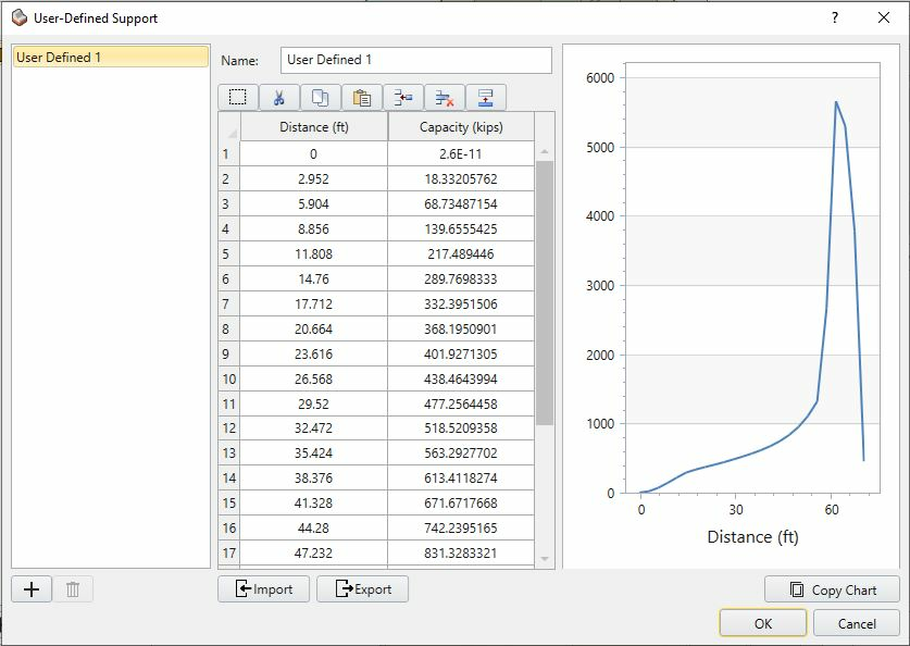
The nonlinear pile capacity envelopes calculated by RSPile were used as inputs in Slide3 to determine user-defined supports. The pile shear resistance against sliding is equal to the shear force from the capacity envelope at the intersection of the slip surface with the pile. The shear force diagram is shown in Fig. 3, where the pile is displaced 1.0 in along its entire length.
The model in Slide3 with the pile spacing dimensions is shown in Fig. 5
Horizontal Spacing = 24 ft
Vertical Spacing = 40 ft
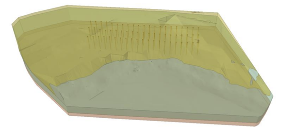
The LEM model with the nonlinear piles was analyzed to find the critical slip surface shown in Fig. 6 with FS= 1.61.
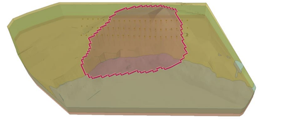
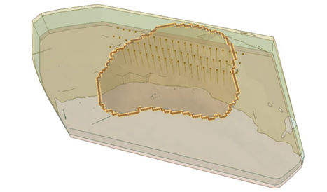
Fig. 7 Shows a clear comparison between the analysis results of the supported slope with nonlinear piles with the unsupported LEM models. The supported slope with nonlinear piles displays major improvement in its stability with a new FS of 1.61. You can see the change in the shape of the critical slip surface between the supported and unsupported LEM models below.

Analysis of the comparison – slope with nonlinear vs constant shear piles
The model was analyzed with the constant shear pile for further comparison, the average capacity was about 1,000 kips computed using the RSPile software. Fig. 8 displays the failure surface with the Spencer FS=1.98 for constant shear piles. In this case, the FS is noticeably higher where the average value of shear resistance capacity is used for piles rather than the nonlinear envelope. The reason for the value being such high is the fact that the point of intersection of critical slip surface varies for different piles. Therefore, the non-linear piles might have the intersection at a lower shear capacity than the average value, which causes a lower FS for the non-linear pile model.
Slide3-RSPile integration model
The new RSPile feature in Slide3 was used to model the piles in the analysis. The pile reactions were calculated directly using RSPile.
For this part of the study, the piles used to reinforce the slope are analyzed using the Finite Element Method (FEM). A coupled procedure is required in which the displacement of the surrounding soil is assumed based on the slipping direction and intersection location of the slip surface with the pile. This displacement is applied to the pile when solving the pile-soil interaction model in RSPile using FEM. Although it is extremely difficult to predict the realistic behaviour of the soil surrounding the pile during mobilization of the soil mass, the displacement magnitude and direction of the soil surrounding the pile are commonly assumed to be uniform above the point of intersection of the slip surface with the pile.
The deformation of the pile because of the soil displacement partitioned along each of its three principal axes (axial direction and the major and minor lateral axes) is obtained via FEM assuming that the pile is a series of discretized deformable elements in an elastic foundation comprising of the surrounding soil.
From the pile analysis results, the internal shear forces of the pile at its intersection with the slipping surface are taken as the restoring reactions of the pile onto the slipping mass in a direction perpendicular to the length of the pile Fig. 9). Similarly, the internal axial force in the pile at the slipping location is taken as a restoring force in the longitudinal direction of the pile. Depending on whether the pile is in tension or compression, the restoring force will be directed into the ground below the slipping surface or in the opposite direction, respectively. Note that in some cases, including both the axial and lateral components of the reaction of the pile may be too conservative. Either of these reactions may be omitted (i.e. taken to be zero) from the analysis if the pile is assumed to be axial- or lateral-only.
The same failure surface was investigated for the Slide3-RSPile integration case as shown in Fig. 8 to see the influence of the analysis pile using RSPile software instead of using the user-defined option.
LEM analysis using the Slide3-RSPile integration feature in Slide3 yields FS = 2.17.
Note that the result differs from the case where user-defined support was used to manually quantify the reaction force because of the following reasons:
- Only the lateral component of the soil displacement is applied during the RSPile analysis
- The effective ground slope varies for each pile, and it is automatically calculated during the RSPile analysis.
These assumptions are not considered in the user-defined result, which makes RSPile analysis more realistic.
Conclusion
Minimizing the potential slope failure hazards is of utmost importance, running an in-depth slope analysis using Rocscience’s Slide3 combined with RSPile for pile capacity can help prevent slope hazards resulting in potential damage to infrastructure.
Read the full study to learn more about this coupled analysis.
