The Power of RS3's Dynamic Analysis in Evaluating Earthquake Response in Residential Buildings
- Sina Moallemi, Geotechnical Product Manager
- Dr. Reginald Hammah, Chief Scientific Officer at Rocscience
To estimate, predict or understand how buildings and other infrastructure respond to earthquakes (seismic loading), geotechnical engineers perform dynamic analysis. Earthquakes generate seismic waves that can cause significant ground motions and damaging outcomes such as soil liquefaction, substantial surface settlement, and foundation and building collapse.
The mechanical properties of soils and buildings significantly influence the dynamic response to seismic (cyclic) loads. These responses can be complex, and their prediction is critical to designing foundations and structures that can resist earthquake forces. Recent events have shown how vital such analysis can be to preventing catastrophic earthquake failures.
The Finite Element Method (FEM) is arguably the most widely applied numerical method in civil and mining engineering. The technique is commonly used in geomechanics to determine the stability of earth walls, embankments, open pits, and underground excavations. It is also used to perform seepage analysis and predict hydraulic structure behaviour. It has been successfully used to perform the dynamic analysis of geotechnical openings and structures to earthquake loads and to design safe systems.
For this article, the 3D FEM software, RS3, was used to demonstrate how to model the response of a six-storey building to earthquake loading (based on the earthquake that occurred in Duzce, Turkey, in 1999). Structural engineers can use the displacements and forces calculated from the analysis to design beams and columns that can safely resist earthquake loads.
Model Description
The model’s geometry, shown in Figure 1, comprises a six-storey building constructed on three layers of relatively weak soil (the total depth is 70m). The Mohr-Coulomb strength properties of the soils are provided in Table 1.
The building has a 10m x 10m base, and each floor is 3-m high. The building’s beams and columns are represented in RS3 with beam elements to capture the axial, lateral and flexural deformations during seismic loading. The beams are assumed to all have 20cm x 40cm cross-sections, while all columns have 50cm x50cm cross-sections. The floor slabs are modelled with 10-cm thick concrete liners.
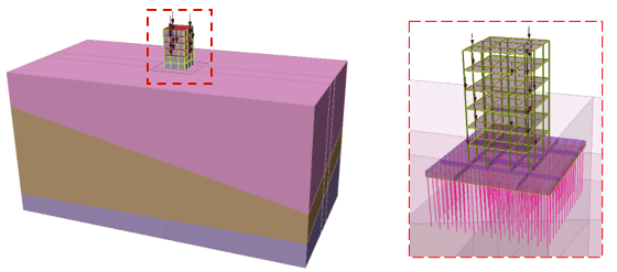
The concrete raft foundation is modelled with a 1-m thick liner/plate. The model assumes that all column-liner and column-beam connections are rigid.
Since the soil layers are weak, the raft is supported on 14-m long piles with 25cm x 25 cm cross-sectional areas. The model assumes that the interface between the soil and the foundation is imperfect and can be characterized by an interface element that allows sliding between the two.
Table 1- Material Properties of Soil Layers |
|||
Top Layer |
Middle Layer |
Bottom Layer |
|
Modulus of Elasticity (kPa) |
50000 |
35000 |
80000 |
Poisson Ration |
0.4 |
0.25 |
0.3 |
Unit weight (kPa) |
27.0 |
24.0 |
27.0 |
Cohesion (kPa) |
10.5 |
5.5 |
12.7 |
Frictional Angel |
35o |
20o |
40o |
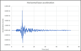
The model was analyzed in two stages. In the first stage, we applied the load case for residential buildings provided in the ACI code to each floor and estimated the initial deformation of the structure. In the second stage, seismic acceleration in the x-direction to the model base was applied. The time history of the seismic acceleration is shown in Figure 2. (Note that the input motion at the model base has a fundamental frequency.)
To correctly predict the behaviour of structures under seismic loading, you need to carefully consider modelling aspects such as the type and location of dynamic boundary conditions, the time steps for implicit time integrations, and damping parameters.
We specified 'transmit' (free field) boundary conditions on the soil layers' vertical, lateral boundaries (surfaces) in the model. This boundary condition absorbs waves originating within the model that reach the lateral surfaces and accounts for free-field motions outside the modelled area. It is appropriate when structures are subjected to earthquake loading (such is our case).
Damping is crucial to predicting the correct response of structures to seismic loads. Damping helps to dissipate energy (a real-world phenomenon) and keep the amplitude of vibrations to realistic ranges. Structural or excavation response to dynamic excitation can be exaggerated without damping, leading to unrealistic (and sometimes unstable) results.
RS3 allows Rayleigh damping, a method that dampens the dynamic response of structures using coefficients proportional to the stiffness and mass of the modelled system. Although very simple, Rayleigh damping can provide a good approximation of the actual damping behaviour of structures. The approach is represented by the simple equation below in which the damping force (and velocity) of the system is expressed solely in terms of the stiffness (K) and mass matrix (M) of the system as:
C= αM+ β K , where α and β are Rayleigh coefficients.
These coefficients are chosen based on the natural frequencies of the system and a desired damping ratio.
The natural frequency and damping of the soil-foundation system can be determined from dynamic analysis. Complete details of such calculations can be found in our dynamic theory manual for RS2/RS3. However, we are providing an overview in this article.
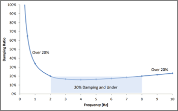
Rayleigh damping allows users to define a damping ratio for a frequency range defined by two frequency values. A curve describes the damping ratios for the remaining frequencies, and this concept is shown in Figure 3 below. All frequencies between the bounding frequencies use the user-specified damping ratio (or lower damping ratios). In contrast, frequencies outside this range are damped more heavily (using the values from the curve).
To establish the two bounding frequencies, we used the method Hudson et al. suggested (1994). According to this approach, we must set the first frequency equal to the natural frequency of soil layers, and the second frequency equal to 𝑛𝜔𝑖. 𝑛 is the closest odd number (not an even number) larger than the ratio, 𝜔𝑖, of the fundamental frequency of the input motion at the model base (which we mentioned earlier) and the natural frequency of the soils in the model.
RS3 has a feature for calculating the natural frequency of the system. For this model, we applied the option and obtained a model natural frequency of 0.83 Hz. Based on the fundamental frequency of the applied acceleration to the base, RS3 calculated an 𝑛 value of 5. Therefore, the second (upper) limiting frequency was 1.128 Hz. To obtain our user-specified damping ratio, we applied the approach suggested by Newmarket and Hall (1982), which uses a value of 0.5% when soil layers are plastic and can considerably dissipate energy during plastic flow.
Using the above recommendations, the Rayleigh damping parameters were estimated as
α=0.0293 (1/s) and β=0.000827 (s)
We used 4-noded tetrahedral elements for the analysis and implicit time integration with a time step of 0.005s. The dynamic analysis was performed for 55 seconds (which matches the duration of the input seismic acceleration time history). We monitored the response of the building structure over this analysis period.
Results
Figure 4 below shows the plot of horizontal displacements with time of three points on the building’s top, middle and bottom floors. The plot shows that the most displacement is observed on the top floor, while the bottom point experiences roughly half of the displacement as the top floor.
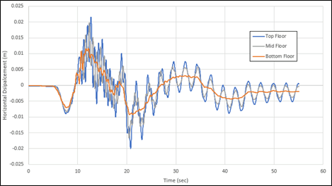
From the motion history of the top and the middle of the structure, we can see the vibrations at a much higher magnitude and frequency than the soil during the first half of the seismic activity. This could cause excessive damage to the structural component if the seismic effects were not accounted for in the design. In this model, all the connections between the column and beam of the structure were assumed fixed and no special treatment for the seismic was accounted for. However, more complicated designs, such as plastic hinge on beam and/or column can be easily incorporated into RS3 to account for the effects of those designs.
In addition to the structural response, the horizontal displacement at each soil layer, underneath the building is plotted in Figure 5. These points are located at Z=0 (the base of the geometry), Z=35m (the middle layer) and Z=70m, (the top layer):
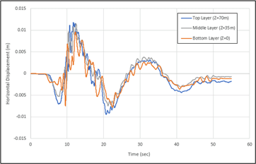
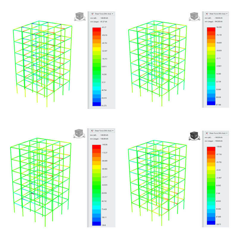
As it can be seen, the behaviour in all layers is very similar which can indicate not much failure occurred in soil layers. However, the transferred seismic load can still have a huge impact on the building. Structural engineers need to know the forces and moments on the building’s structural components to design them to resist the earthquake loads safely. Figure 6 shows the shear force distributions in the beams and columns of the structure at four different time steps: T=0 (top left), 10 sec (top right), 15 sec (bottom left) and 18 sec (bottom right).
Concluding Remarks
The purpose of this article is to describe a simple example illustrating RS3’s capabilities to perform dynamic analysis of geotechnical structures and excavations under earthquake loadings. RS3 offers a comprehensive and intuitive suite of analysis tools that you can use to investigate engineering performance under the most challenging seismic conditions.