Advancing Slope Stability Analysis with Probabilistic Methods in Slide2 and Slide3
In a past webinar, Dr. Sina Javankhoshdel (Senior Manager - LEM) detailed how adding statistical rigor to slope stability analysis can improve risk assessment. This article distils the key outcomes from the webinar into actionable steps for defining input probability distributions, running probabilistic simulations, and calibrating models to field observations using Slide2 and Slide3.
Why Probabilistic Analysis Matters
Real-world geotechnical parameters are rarely single, unique values; there is always uncertainty associated with them. Probabilistic methods address these uncertainties in input parameters (e.g., cohesion, friction angle) by assigning statistical distributions to them. This approach leads to the calculation of outcome probabilities instead of relying solely on one value, such as a factor of safety (FoS). For example, in slope performance, you can derive a probability of failure, Pf (i.e., the likelihood of a factor of safety being less than 1), and quantify your confidence.
As Sina emphasized, "Incorporating variability transforms our models from conservative guesses into risk-informed decision tools."
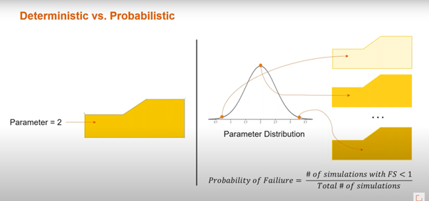
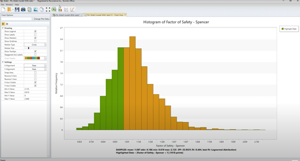
Slide2 and Slide3 allow users to define statistical parameters such as mean, standard deviation, and distribution type (e.g., normal, log-normal, uniform) for input variables. Sampling methods like Monte Carlo, Latin Hypercube and Response Surface are then employed to generate numerous realizations of these parameters. Each realization set is used to compute a FoS, and the entire complement produces a histogram of FoS values.
The Pf is then calculated as the proportion of simulations in which FoS < 1, providing a quantitative measure of risk.
Why use the Stochastic Response Surface Method (SRSM) over Monte Carlo or Latin Hypercube?
One of the challenges in probabilistic analysis is the computational cost of running thousands of slope stability simulations. The SRSM addresses this limitation by using machine learning to approximate the relationship between input parameters and FoS. In SRSM, a smaller subset of simulations is run to train a response surface model, which then predicts FoS for the complete set of samples. This approach dramatically reduces computation time—from hours or days to minutes—while maintaining accuracy close to that of the traditional probabilistic methods. Users can set up SRSM in Slide3 by selecting it as the sampling method (under Project Settings) and specifying the desired number of samples.
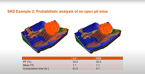
To demonstrate the efficiency of SRSM, it was compared to the traditional Latin Hypercube method using a model with 3,000 simulations. While the Latin Hypercube method used 62 hours of computation, SRSM completed the same analysis in just 4 hours with similar mean factor of safety of 1.1 (Figure 3). In another example involving a 2D slope with a weak layer and variable load, SRSM achieved identical probability of failure results to the Latin Hypercube method in just a fraction of the time.
Back Analysis Using Probabilistic Methods
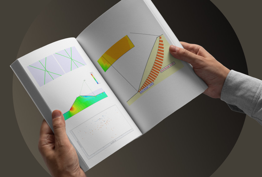
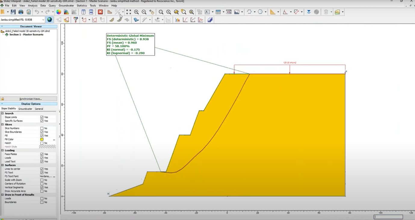
Back analysis is a powerful technique for calibrating material properties based on observed slope failures. When the failure surface is known, engineers can use Slide2 and Slide3 to estimate the range of material parameters consistent with the failure. The back analysis workflow starts with importing an actual failure surface and specifying it as a user-defined slip surface. It then runs a probabilistic analysis with uniform distributions for the input parameters. (The latter setting ensures that all parameter values are considered equally.) Scatter plots showing combinations of cohesion and friction angle that yield FoS around 1 can be used to identify plausible material properties that led to the failure (Figure 4).

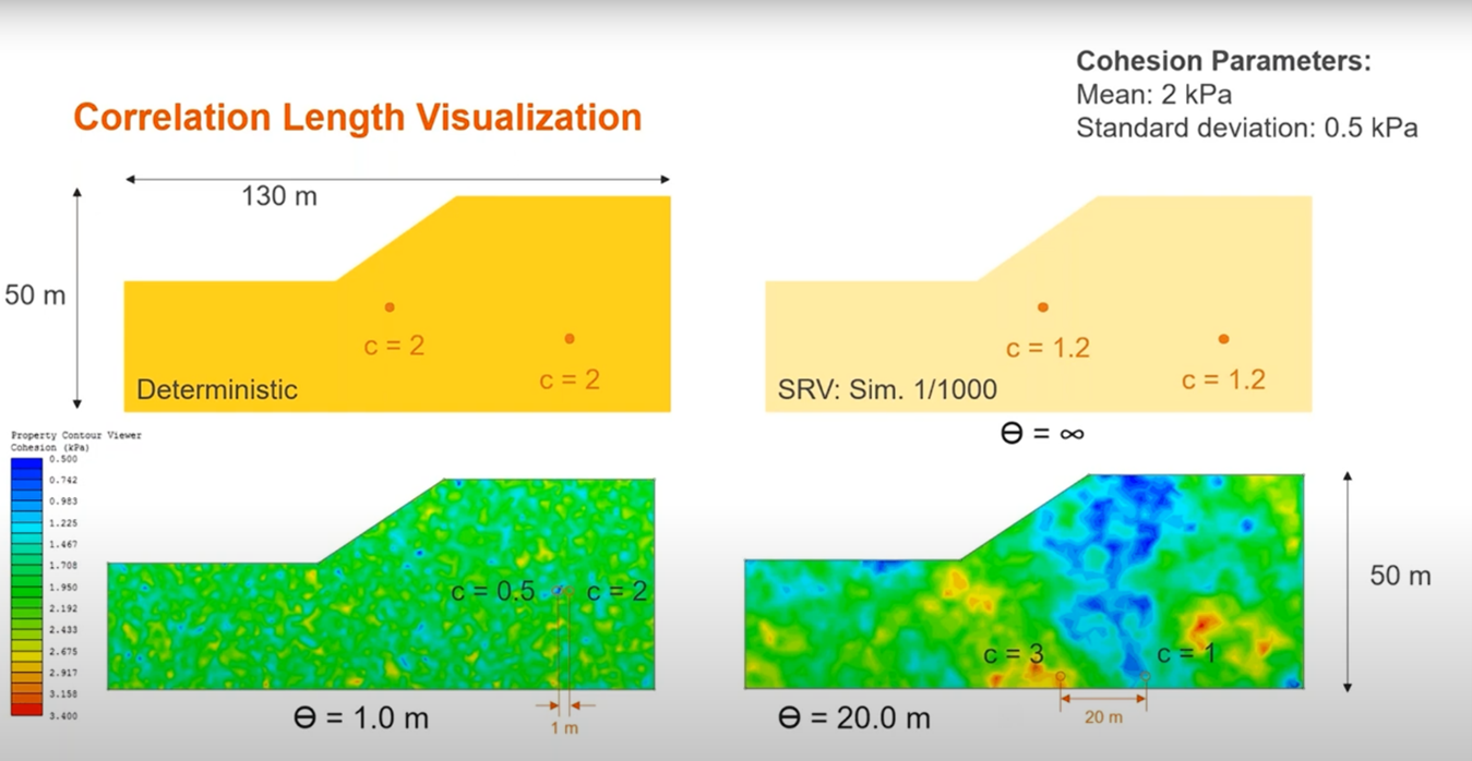
Spatial Variability and Advanced Modeling
In the real world, soil properties vary spatially. Slide2 offers a spatial variability feature that allows users to capture this critical aspect. The feature enables users to generate parameters that change with location according to defined spatial correlation lengths. This feature generates multiple spatially variable fields for simulations that capture realistic heterogeneity in soil profiles. Combining spatial variability with non-circular search methods and surface-altering optimization enables the identification of failure surfaces that follow weak zones. This feature improves the reliability of stability assessments.
Integration Between Slide2 and Slide3
Rocscience software enables users to integrate their Slide2 and Slide3 analyses seamlessly. For example, users can export probabilistic models and spatial fields as discrete functions that allow advanced 3D modelling with spatial variability. This integration facilitates comprehensive analyses even with complex geometries and boundary conditions (such as spaced relief wells in levees).
In Summary
- Use probabilistic analysis to quantify risks and inform design decisions beyond traditional FoS values.
- Employ SRSM for efficient model setup and sensitivity studies, followed by full Latin Hypercube simulations for final verification.
- Apply back analysis to calibrate soil parameters from known failures, improving model accuracy.
- Incorporate spatial variability for a realistic representation of soil heterogeneity.
- Leverage Slide2 and Slide3 integration for advanced 3D probabilistic modelling.