5 - Rigid Analysis of Polygonal Pillar

In Tutorial 01 - Quick Start (Rigid Analysis of Square Pillar), you learned about the Rigid analysis method in CPillar for a Rectangular Pillar with vertical abutments. In this tutorial, you will learn how to define the geometry and lateral stress orientations for a Polygonal Pillar with non-vertical abutments.

Topics Covered in this Tutorial:

• Project Settings
• Rigid Analysis for Polygonal Pillar
• Non-vertical Abutments
• Principal Stresses
• Deterministic Analysis
• Input Data
• Analysis Results
• Mohr-Coulomb Strength Criterion
• Water Pressure
• Sensitivity Analysis

Finished Product:

The finished product of this tutorial can be found in the Tutorial 05 Rigid Analysis of Polygonal Pillar.cpil5 file, located in the Examples > Tutorials folder in your CPillar installation folder.

1.0 Introduction

This model represents a Polygonal Pillar with a thickness of 4 meters. There is 1 meter of overburden and 1 meter of free water (6 – (4+1) = 1).

The lateral stress is defined by gravity. Lateral stresses will be calculated based on the horizontal/vertical stress ratios.

2.0 Creating a New File

If you have not already done so, run the CPillar program by double-clicking the CPillar icon in your installation folder or by selecting Programs > Rocscience > CPillar > CPillar in the Windows Start menu.

When the program starts, a default model is automatically created. If you do NOT see a model on your screen:

• Select: File > New

Whenever a new file is created, the default input data forms valid pillar geometry, as shown in the image below.

If the CPillar application window is not already maximized, maximize it now so that the full screen is available for viewing the model. You will have a 3D pillar displayed on the screen in isometric orientation.

3.0 Project Settings

The Project Settings dialog allows you to configure the main analysis parameters for your model, such as Units, Analysis Type, and Sampling Method.

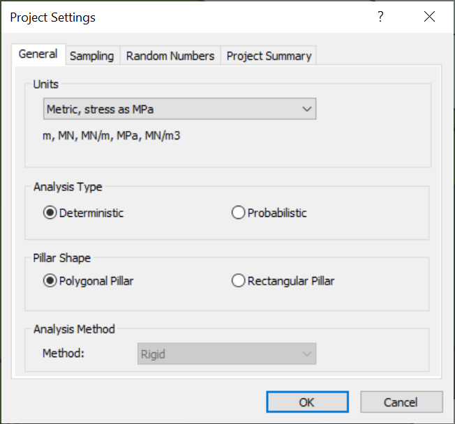
3.1 General

1. Select Project Settings from the toolbar or the Analysis menu.
   
2. Navigate to the General tab of the Project Settings dialog.
3. Ensure Units = Metric, stress as MPa (default setting).
4. Set Analysis Type = Deterministic.
5. Set Pillar Shape = Polygonal Pillar.
   
   

3.2 Project Summary

1. Navigate to the Project Summary tab of the Project Settings dialog.
2. Enter CPillar Rigid Analysis of Polygonal Pillar Tutorial as the Project Title.
   
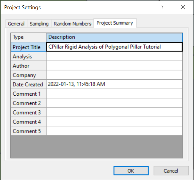
3. Click OK to close the Project Settings dialog.

4.0 Stope Section Geometry

Unlike a Rectangular Pillar stope section which is defined by a Pillar Length and Pillar Width, a Polygonal Pillar is defined by at least 3 vertices (x, y). The 2D stope section geometry is defined in the Stope Section view. Let's switch to the Stope Section view.

To access the Stope Section view:

• Select Stope Section from the toolbar dropdown, or from the Select View submenu of the View menu.

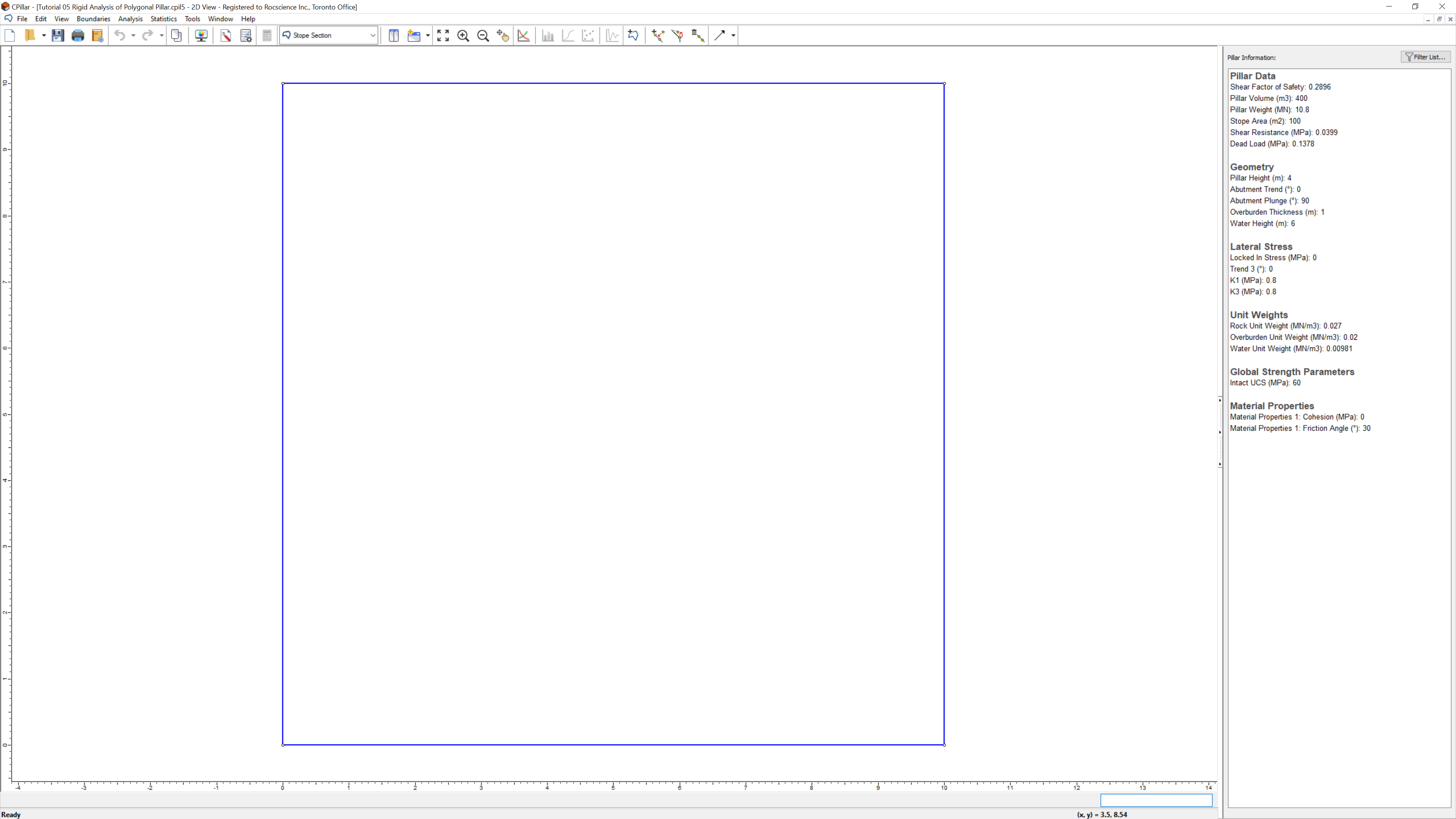
By default, four vertices define a 10 by 10 square pillar in the Stope Section view.

The 2D coordinates of the Stope Section can be defined in three ways:

• Imported from a 2D DXF file, using Import DXF option in the File > Import menu.
• Graphically, using Add Stope Section option from the toolbar, Boundaries menu, or right-click menu.
• In a table of x and y coordinates, use the Edit Coordinates option from the Boundaries > Edit menu, or right-click menu.

To define the geometry of the polygonal pillar:

1. Select Add Stope Section option from the toolbar, Boundaries menu, or right-click menu.
The previous stope section geometry is deleted and the cursor turns into a crosshair allowing you to start drawing. If you cancel or enter an invalid polygon, the stope section geometry will be reverted back.
2. Enter the following coordinate pairs in the prompt line at the bottom right of the screen. The X and Y coordinates can be separated by a space or a comma. Press ENTER at the end of each pair/line.

Point	Easting (X)	Northing (Y)
1	0	0
2	-1	1
3	-2	5
4	6	8
5	7	4
6	3	1
7	2	-3
8	1	-4

3. Type c in the prompt line and press ENTER to automatically close the polygon.

The Stope Section view shows the 2D geometry of the top of the polygonal stope section:

5.0 Input Data

In CPillar, the input parameters are entered in the Input Data dialog. The Input Data dialog is organized under four tabs: Geometry, Stresses, Material Properties, and Rock Mass and Abutment Strength. To change a parameter, click on the value and enter the new value or select from the dropdown as necessary. The model will reflect any changes, immediately. Mean values are entered directly in the edit controls in the Input Data dialog.

5.1 Geometry

To set up the analysis in the Input Data dialog:

1. Select Input Data from the toolbar or Analysis menu.
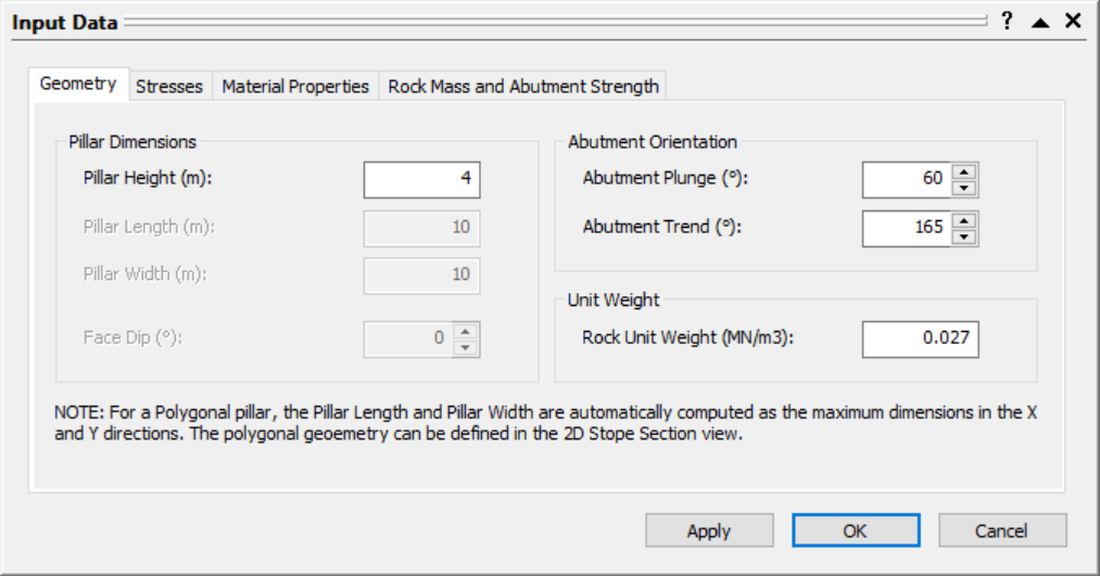
2. Navigate to the Geometry tab.
3. Enter the following data for the Pillar Dimension parameter:
   • Pillar Height = 4 m.
4. Enter the following mean data for the Abutment Orientation parameters:
   • Abutment Plunge = 60 deg
   • Abutment Trend = 165 deg
5. Enter the following mean data for the Unit Weight parameter:
   • Rock Unit Weight = 0.027 MN/m3
     
     

5.2 Stresses

Enter the following mean data for the stress parameters:

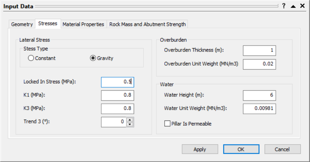
1. Navigate to the Stresses tab of the Input Data dialog.
2. Enter the following mean data for the Lateral Stress parameters:
   • Stress Type = Gravity
   • Locked In Stress = 0.5 MPa
   • K1 = 0.8
   • K3 = 0.8
   • Trend 3 = 0 deg
3. Enter the following mean data for the Overburden parameters:
   • Overburden Thickness = 1 m
   • Overburden Unit Weight = 0.02 MN/m3
4. Enter the following mean data for the Water parameters:
   • Water Height = 6 m
   • Water Unit Weight = 0.0098 MN/m3
   • Pillar Is Permeable = No
     
     

5.3 Material Properties

The pillar overlies a region containing two different rock types:

• The hang wall comprises granite with a high friction angle
• The footwall and sidewall comprise of weak schist with a low friction angle

We will define two different Material Properties with different shear strength parameters:

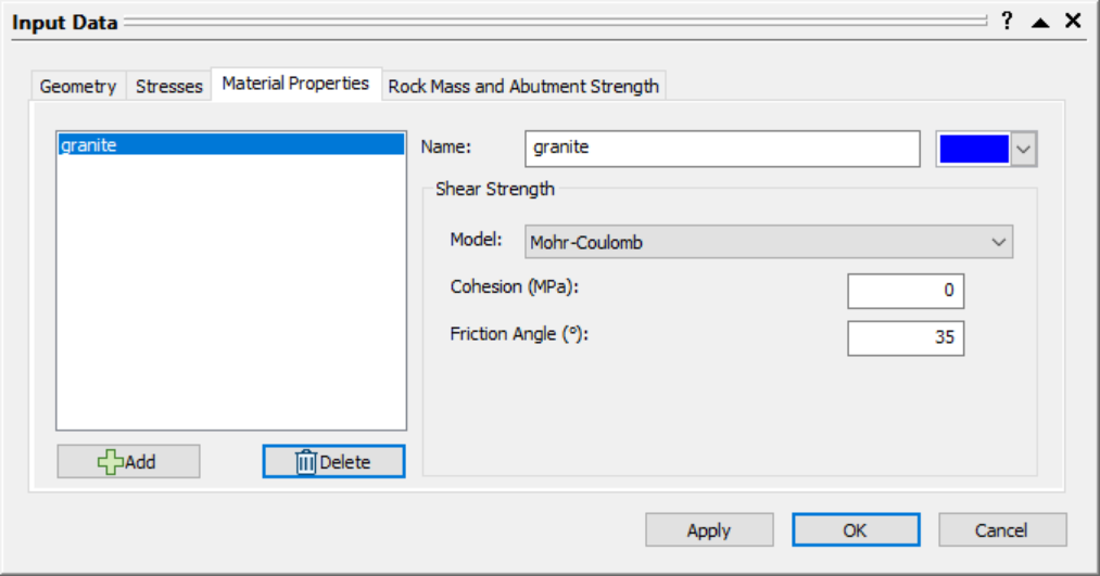
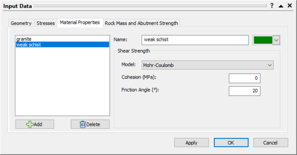
1. Navigate to the Material Properties tab of the Input Data dialog.
2. Set the Name = granite and enter the following Shear Strength parameters:
   • Strength Type = Mohr-Coulomb
   • Cohesion = 0 MPa
   • Friction Angle = 35 deg
     
3. Select the Add button to add another material property.
4. Set the Name = weak schist and enter the following Shear Strength parameters:
   • Strength Type = Mohr-Coulomb
   • Cohesion = 0 MPa
   • Friction Angle = 20 deg
     

5.4 Rock Mass and Abutment Strength

Enter the following mean data for the rock mass parameters:

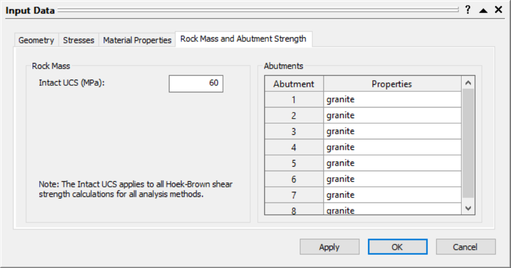
1. Navigate to the Rock Mass and Abutment Strength tab of the Input Data dialog.
2. Enter the following mean data for the Rock Mass parameter:
   • Intact UCS = 60 MPa
3. By default, Abutments are assigned the first Property (i.e., granite). You can reassign Abutments to another Property by clicking on the dropdown. We will leave it as is in the Input Dialog, and assign materials graphically in the next steps.
   
4. Click OK to apply the changes and close the dialog.

6.0 Assign Material Properties

While in the Stope Section view, to assign Material Properties graphically:

1. Select Assign Materials from the Boundaries menu or right-click menu.
2. Select weak schist from the list in the Assign Material dialog.
   
   
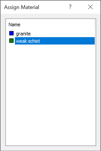
3. Left-click on the longest segment between vertex 3 (-2, 5) and vertex 4 (6, 8). Abutment 3 has been assigned to weak schist material.
4. Click X to close the Assign Material dialog, or right-click and select Done to finish assigning materials.

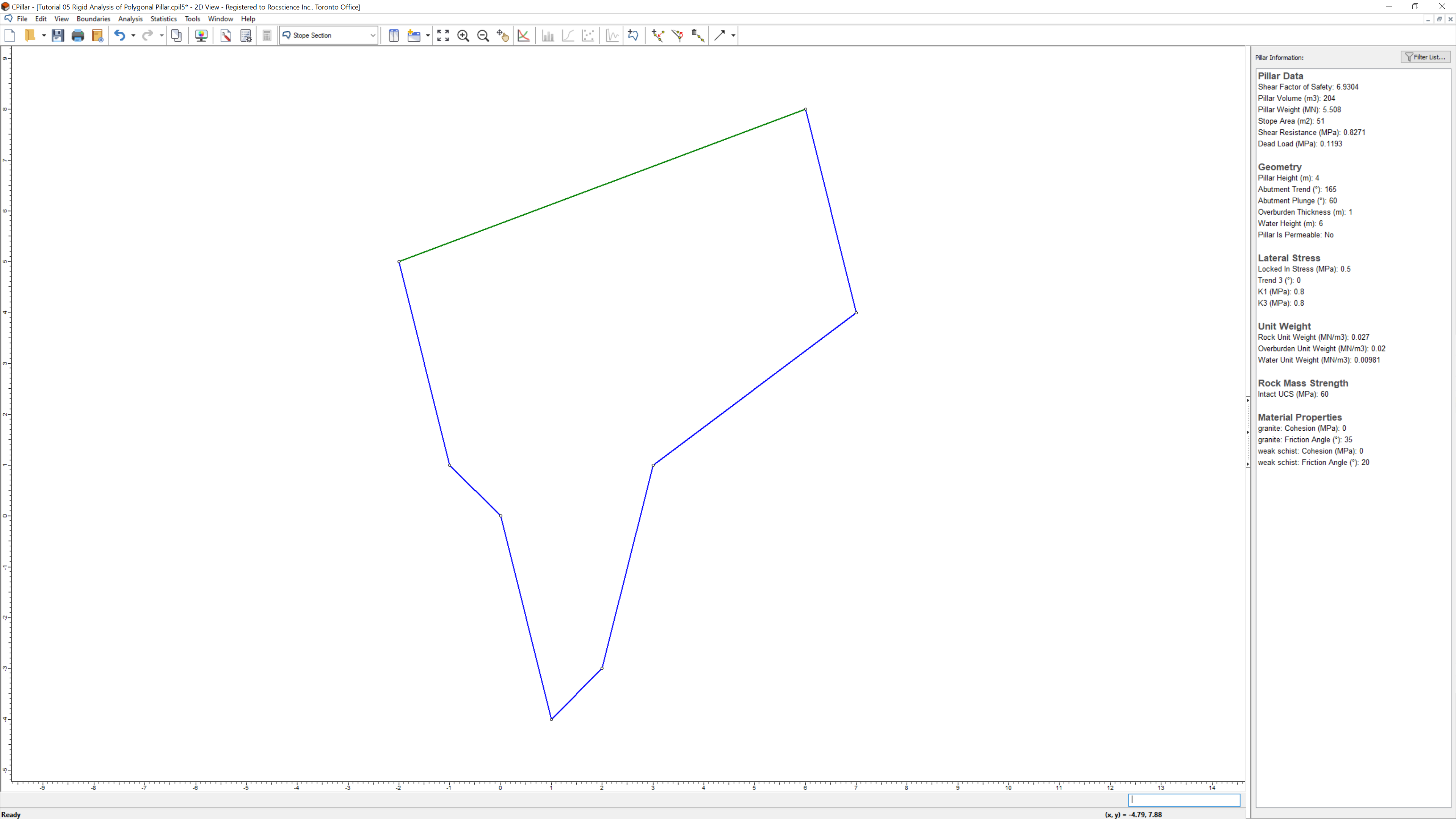
The Stope Section view shows the 2D geometry of the top of the polygonal stope section with weak schist material property assigned to the northwest hang wall:

A number of annotation tools are also available in the toolbar or Tools menu. See the Drawing Tools topic for more information.

Switch back to the 3D Pillar View:

• Select 3D Pillar View from the toolbar dropdown, or from View > Select View.
  

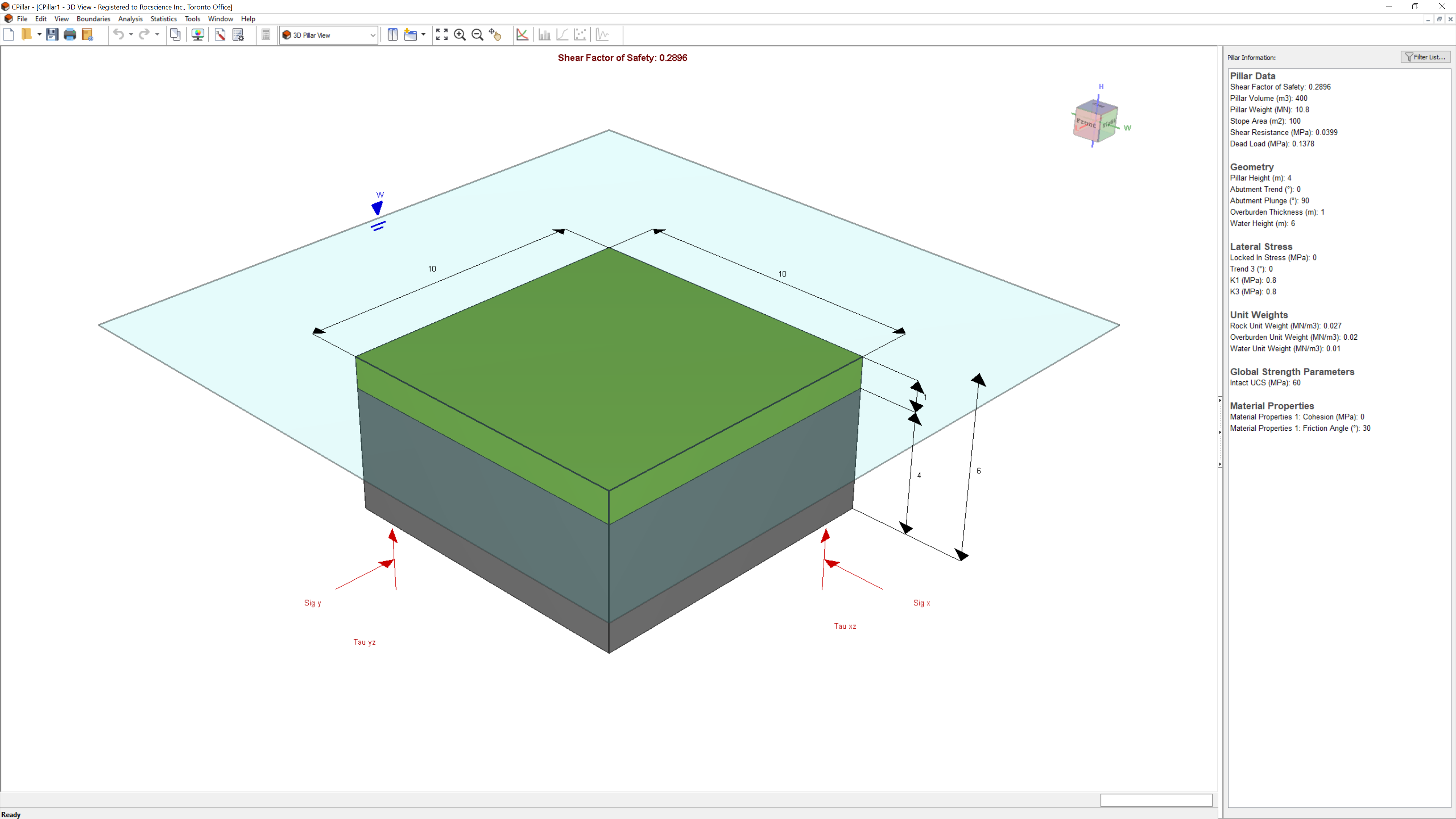
The 3D Pillar View shows an isometric perspective of a 3D pillar model with principal stresses and dimensions labelled:

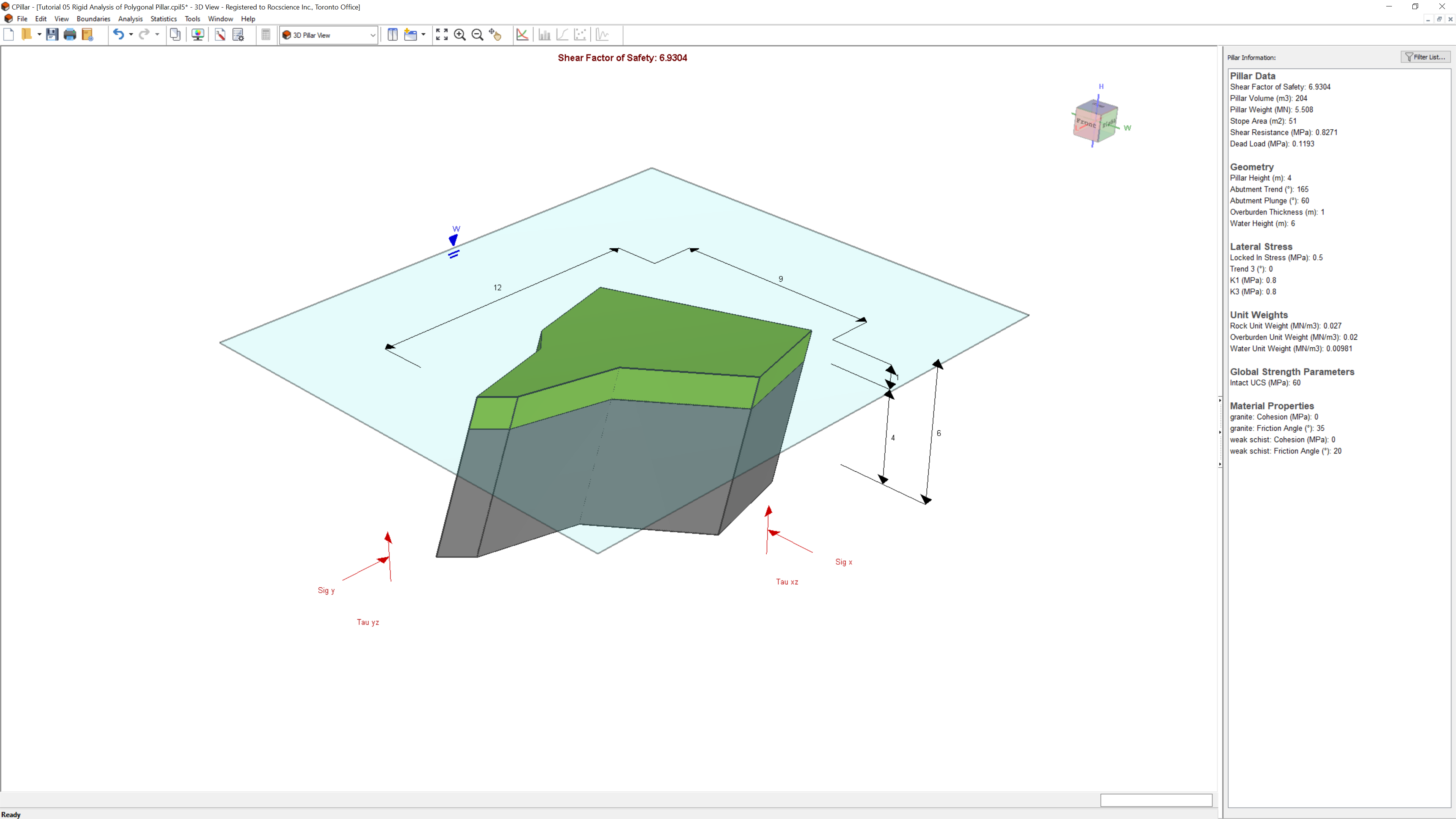
Notice that the abutments are no longer vertical. The slippage along the abutments occurs at a 60-degree angle from the horizontal.

7.0 Analysis Results

To ensure the latest analysis results are always displayed, CPillar automatically computes an analysis whenever:

• A file is opened, or
• Input data is entered or modified in the Input Data dialog.

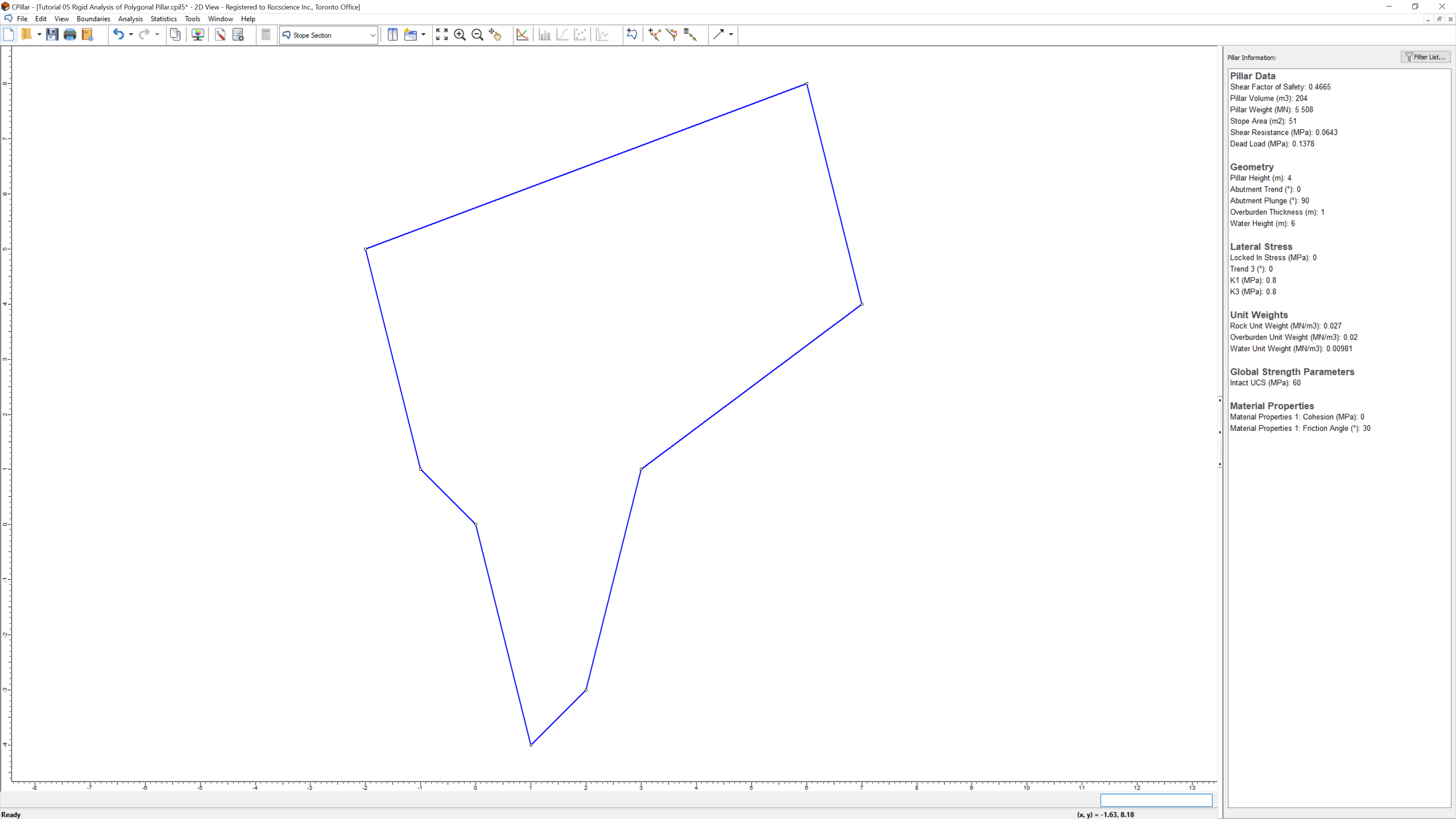
The primary result from a CPillar Deterministic Analysis is the pillar Factor of Safety. The Factor of Safety is displayed at the top-center of the 3D Pillar View and in the Pillar Information pane. The Pillar Information pane appears in the Sidebar on the right side of the CPillar application window and displays a summary of analysis results.

Note that, since this is a Rigid analysis, shear is the only failure mode; as such shear is the only failure result displayed. The Shear Factor of Safety is 6.9304.

8.0 Sensitivity Analysis

The final section of the tutorial demonstrates the CPillar Sensitivity Analysis feature. In a Sensitivity Analysis, individual variables can be varied among user-defined minimum and maximum values while all other input parameters remain constant. This allows you to determine the effect of individual variables on the Factor of Safety.

We will use Sensitivity Analysis to show the effects of abutment and stress orientation on the Factor of Safety.

1. Select Sensitivity Analysis on the toolbar or on the Analysis menu.
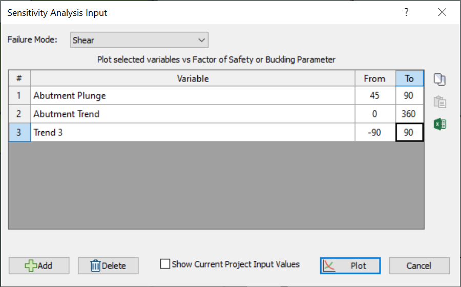
2. In the Sensitivity Analysis Input dialog:
   • Select the Add button in the Sensitivity Analysis Input dialog then select Abutment Plunge from the drop-down list.
   • Enter Abutment Plunge From = 45 and To = 90 deg.
   • Select the Add button in the Sensitivity Analysis Input dialog then select Abutment Trend from the drop-down list.
   • Enter Abutment Trend From = 0 and To = 360 deg.
   • Select the Add button in the Sensitivity Analysis Input dialog then select Trend 3 from the drop-down list.
   • Enter Trend 3 From = -90 and To = 90 deg.
     
3. Click Plot.

You should see the following Sensitivity Plot:

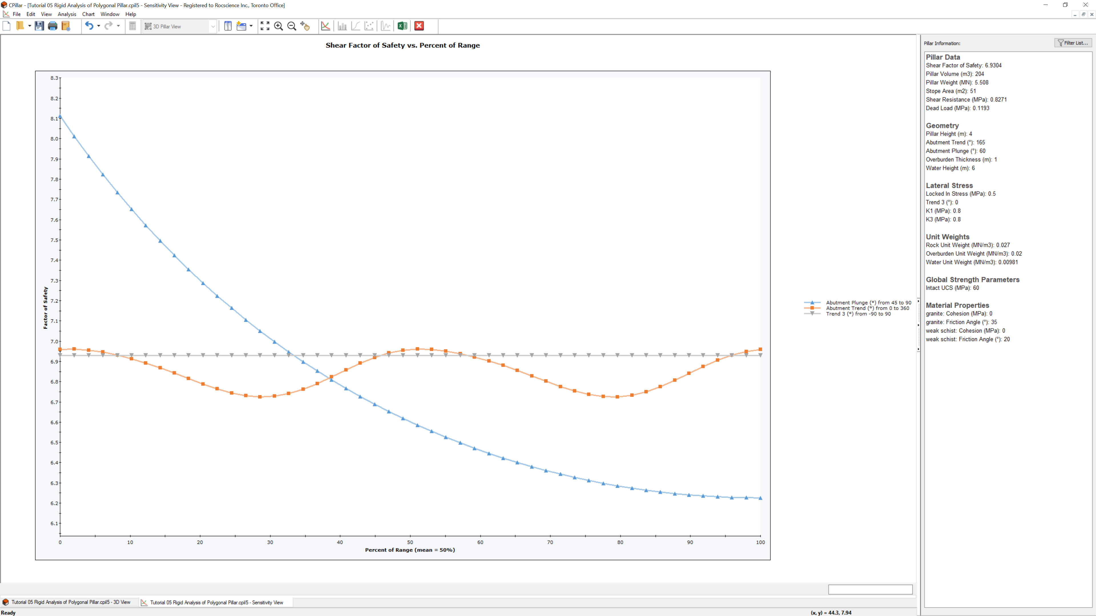
Notice that the Factor of Safety follows a sinusoidal relationship with respect to Abutment Trend with a period of 180 degrees. This is due to the fact the shear strength is the same when the abutment is slanting in the opposite Abutment Trend direction. The Factor of Safety decreases to the minimum actor of Safety as the Abutment Plunge approaches 90 degrees (i.e., vertical) as driving forces increase and normal forces along the abutments decrease.

Trend 3 orientation (of principal stress Sigma3) has no impact on the Factor of Safety since K1 = K3 (i.e., isotropic soil stress behaviour).

This concludes the tutorial.