The Mechanics of Pile Downdrag: Field Evidence and 3D Analysis in RS3
- Sina Moallemi, Geotechnical Product Manager
How much drag force should be considered when designing a pile subjected to settlement? It is a deceptively simple question, but the answer can influence the geotechnical ultimate limit state (ULS) design of a pile.
When soil settles relative to a pile, negative skin friction develops along the shaft, generating a downward force known as drag force. How this force is treated in geotechnical ULS design, however, depends on the governing design code. AASHTO includes drag force as an applied load and excludes the shaft resistance above the neutral plane from the pile's resistance. The Canadian Highway Bridge Design Code (CHBDC), in contrast, does not include drag force in its geotechnical ULS calculations.
These differences can lead to different design outcomes, even under comparable ground conditions. But how significant is the effect of drag force in practice, and what happens when the pile's actual response is considered?
A field study at the Daly Overpass in Brandon, Manitoba, offered an opportunity to look beyond the assumptions embedded in either approach. By combining full-scale field measurements, dynamic pile testing and 3D finite element analysis in RS3, Chalajour, Blatz and Bartz investigated how drag force developed in an instrumented pile and what that meant for ULS design under the two codes.
The study provides a detailed look at how the pile, soil and embankment interacted over time – and how those interactions influenced the resulting design assessments.
Site Conditions and Instrumentation
The Daly Overpass is a four-lane bridge in Brandon, Manitoba, Canada, completed in 2024. For the field study, the researchers selected a steel HP 310 × 110 pile, driven to a depth of approximately 37 m at the corner of the bridge abutment foundation.
The pile was adjacent to a mechanically stabilized earth (MSE) wall, with approximately 9 m of backfill extending 100 m behind the abutment. The site profile consisted of approximately 1.5 m of clayey sand over glacial clay till, with shale bedrock at approximately 40 m depth.
The site presented the conditions needed to investigate negative skin friction: a compressible soil profile, substantial embankment loading and the gradual consolidation that follows construction. Rather than relying solely on assumed soil movements, the researchers instrumented the pile to observe how the ground and foundation responded over time.
Ten pairs of vibrating wire strain gauges were installed along the upper half of the pile to measure changes in axial force. Piezometers at depths of 13, 23 and 33 m monitored groundwater conditions and pore-water pressure. Together, these instruments provided a record of pile loading and the surrounding soil's response as construction progressed.
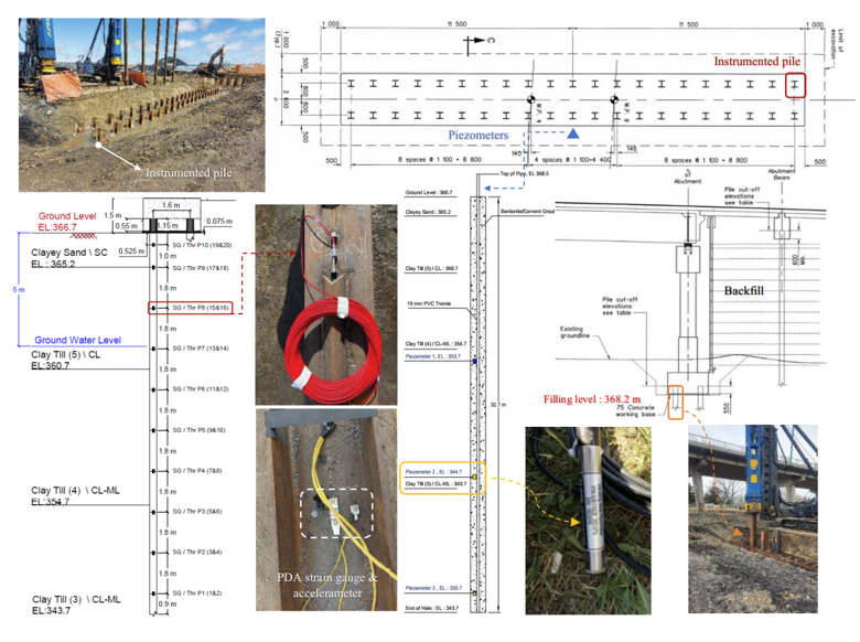
Field measurements continued for more than two years after pile installation. This allowed the researchers to examine the effects of several construction stages, from abutment column construction and embankment filling to consolidation and the application of bridge dead load.
Establishing Pile Capacity
Before investigating long-term drag force, the researchers needed to understand how the pile's axial capacity developed after installation.
Dynamic testing was conducted during pile driving and through three subsequent restrike tests. Measurements from a pile driving analyzer were interpreted using the Case Pile Wave Analysis Program (CAPWAP) to estimate the pile's shaft and tip resistance.
At the end of initial driving (EOID), the pile's total capacity was 2,233 kN. Subsequent restrike tests showed a steady increase, reaching 2,970 kN at the third restrike, approximately 21.5 hours after EOID. This represented an increase of about 33%, primarily due to shaft setup.
- First restrike: 2,547 kN, 15 minutes after EOID
- Second restrike: 2,760 kN, 135 minutes after EOID
- Third restrike: 2,970 kN, 21.5 hours after EOID
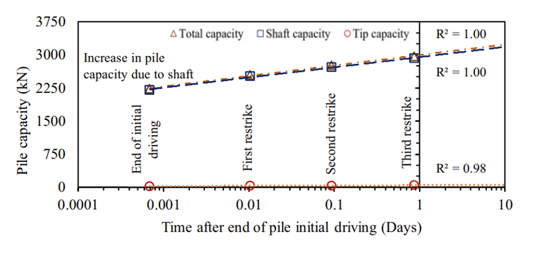
The increase highlights an important consideration in pile design: resistance measured immediately after driving may differ from resistance mobilized after installation. However, capacity testing alone could not establish how much settlement-induced drag developed along the pile or where the transition between negative and positive shaft friction occurred.
That required an analysis of the relative movement of the pile and surrounding soil.
Reconstructing Construction and Consolidation in RS3
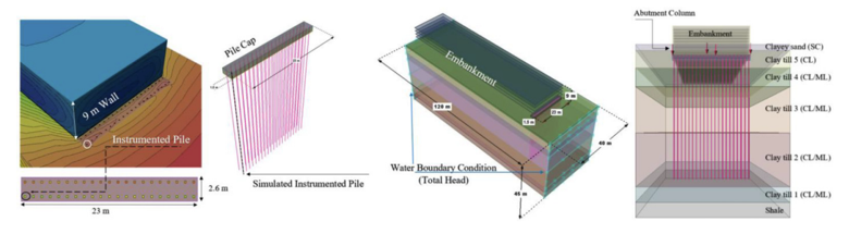
The researchers used RS3 to model the pile, surrounding soil and construction sequence in three dimensions. Rather than treating the final condition as a single loading state, the analysis reproduced the main stages of construction and consolidation observed at the site.
The sequence included:
- Establishing in-situ conditions and activating the pile and pile cap.
- Applying the column load to the pile cap over 20 days.
- Allowing 90 days for consolidation.
- Constructing the 9 m embankment in 0.225 m lifts over 40 days.
- Allowing a further 160 days for consolidation.
- Applying the bridge dead load over 60 days.
- Continuing the consolidation analysis.
This staging was important because drag force depends on the relative movement of the pile and surrounding soil. The model therefore needed to capture not only the loads applied to the pile, but also how the ground responded to those loads over time.
The embankment fill, clay till and sandy layers were represented using the Mohr–Coulomb elastic-perfectly plastic material model. The clay was modelled as undrained during loading to account for excess pore-water pressure dissipation over time, while the sand was modelled as drained.
The pile was represented using linear elastic beam elements with an elastic modulus of 210 GPa. Its connection to the pile cap was fixed to account for bending, while the soil-pile interface was modelled using the Mohr-Coulomb failure criterion with an interface friction coefficient of 0.7.
The analysis did not simulate the short-term pore-pressure effects of pile driving; these were assumed to have dissipated before embankment loading began.
Putting the Model to the Test
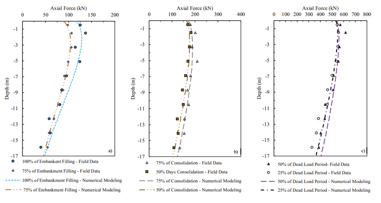
A numerical model is only useful if it can reasonably reproduce the behaviour observed in the field. The researchers therefore compared the RS3 results with measurements collected during construction and consolidation.
The comparison showed reasonable agreement between modelled and measured axial force distributions across the key stages of embankment filling, post-fill consolidation and dead-load application.
The researchers also compared modelled and measured total water head at the 13 m and 23 m piezometer depths. This provided an additional check on the model's representation of groundwater response and consolidation.
The researchers also compared modelled and measured total water head at the 13 m and 23 m piezometer depths. This provided an additional check on the model's representation of groundwater response and consolidation.
Together, these comparisons supported the use of the numerical model to investigate the longer-term behaviour of the pile, including the location of the neutral plane and the resulting drag force.
Finding the Neutral Plane
As soil settles relative to a pile, the direction of shaft friction changes along its length. Above the neutral plane, the settling soil moves downward relative to the pile, generating negative skin friction. Below it, the pile moves downward relative to the soil, mobilizing positive shaft resistance.
The neutral plane marks the depth at which the pile and surrounding soil settle equally. Its location is therefore central to evaluating drag force and the pile's axial load distribution.
The RS3 analysis showed that the neutral plane changed position throughout construction and consolidation. Following embankment filling, it moved down to approximately 2–3.5 m during the subsequent consolidation period. Application of the bridge dead load shifted it upwards, to approximately 1.5 m below the pile head, before it gradually moved downward again as consolidation continued.
At steady state, the neutral plane was located approximately 9 m below the pile top. The maximum axial force along the pile reached 620 kN, while the calculated drag force was 70 kN. The analysis also predicted 8 mm of relative soil-pile settlement and 23 mm of pile downdrag.
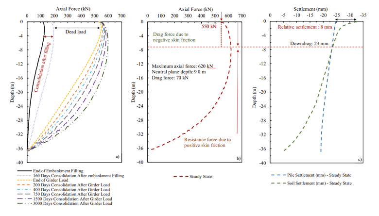
These results show why the neutral plane cannot simply be assumed from the soil profile or the depth of the settling layer. Its position depends on the relative deformation of the pile and surrounding ground as loading and consolidation progress.
For this floating friction pile in compressible clay till, the analysis predicted a relatively small drag force. The authors also note that piles with greater end-bearing resistance can experience different soil–pile settlement patterns and larger drag forces.
Bringing the Results Back to Design
With the pile capacity and drag force evaluated, the researchers compared the geotechnical ULS requirements under AASHTO conditions C1 and C2 and CHBDC ULS Combination 2.
The comparison considered the applied dead, live and soil loads, bearing friction and the treatment of drag force. Under AASHTO, shaft resistance above the neutral plane was excluded from the resistance used in the ULS calculation, while drag force was incorporated into the applied load. CHBDC did not include drag force in its geotechnical ULS calculation.
The final restrike results are summarized below.
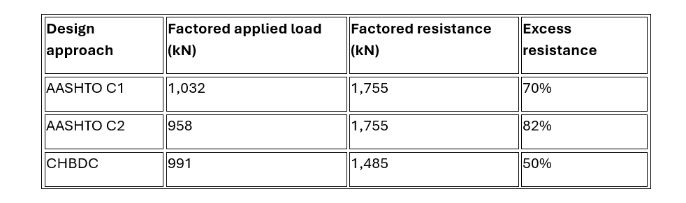
The excess resistance represents the difference between factored resistance and factored applied load, expressed as a percentage of the applied load.
All three design approaches satisfied the geotechnical ULS requirements for the pile. However, CHBDC produced the most conservative result in this case, with a 50% excess resistance compared with 70% for AASHTO C1 and 82% for AASHTO C2.
This outcome is notable because AASHTO explicitly includes drag force in its ULS calculation, whereas CHBDC does not. The difference was largely attributable to the dynamic resistance factors used in the comparison: 0.65 for AASHTO and 0.50 for CHBDC.
The result should be understood in the context of the site conditions investigated. The calculated drag force was relatively small, and the neutral plane was close to the pile head compared with the overall pile length. The authors note that where drag force is more significant, such as in piles with hard end-bearing conditions, AASHTO predictions may be lower than those from CHBDC.
The comparison therefore demonstrates that the treatment of drag force cannot be considered in isolation. Its magnitude, the neutral plane location, the available pile resistance and the load and resistance factors in the governing code all influence the ULS outcome.
From Field Evidence to Engineering Decisions
The Daly Overpass study brought together three complementary sources of evidence: long-term field monitoring, dynamic pile testing and 3D numerical modelling.
Field instrumentation captured changes in axial force and groundwater conditions. Dynamic testing established how pile capacity evolved after driving. RS3 reproduced the construction and consolidation sequence, allowing the researchers to investigate soil–pile interaction, track the neutral plane and quantify drag force.
For the pile investigated, the analysis predicted a 70 kN drag force and a steady-state neutral plane approximately 9 m below the pile top. The model's agreement with field measurements provided a basis for examining how these results influenced ULS design under AASHTO and CHBDC.
The broader engineering lesson is that code provisions define how loads and resistance are treated in design, but evaluating settlement-induced drag requires an understanding of how the soil–pile system behaves. By connecting field observations with dynamic testing and numerical analysis, engineers can examine the mechanisms behind the design values and make more informed assessments of pile performance.
Model Complex Soil–Structure Interaction in RS3
Simulate staged construction, consolidation, and 3D pile–soil behaviour to evaluate neutral plane depth and drag forces with confidence.
Start Your Free Trial