Rocscience FEM Software: Now More Powerful and Flexible Than Ever
This Spring will see new releases of Rocscience’s robust FEM software products, RS2 and RS3. In RS2, you can look forward to powerful new features, including a brand new Dynamic Data Analysis option, the addition of the Finn material model to enable more accurate analysis of pore pressure build-up under seismic conditions, and two new Dynamic Boundary Condition types for even more realistic Dynamic Analysis of dams and embankments. In RS3 you’ll find a new Shear Strength Reduction Graph. Keep reading to get all the details.
Dynamic Data Analysis in RS2
An accurate and efficient Dynamic Analysis of your model starts with the quality of your time history input data. That is why RS2 now features a new Dynamic Data Analysis option. When defining a Dynamic Load, you can now use the option to view, analyze, and filter load function input data before adding the load to your model.
Dynamic Data Analysis Dialog
At the core of the new option is the Dynamic Data Analysis dialog, which you can use to create a Dynamic Load Function. Once you create the function, you can assign it to one or more Dynamic Loads. To open the dialog, select Dynamic Data Analysis from the toolbar or the Dynamic menu.
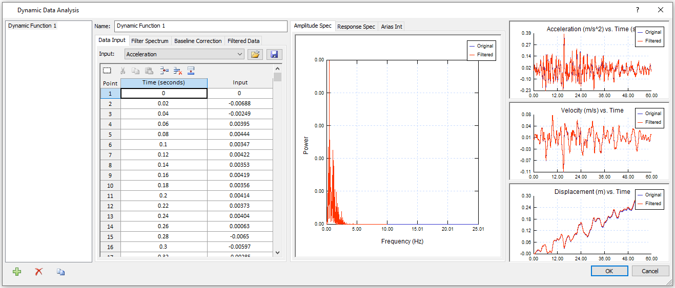
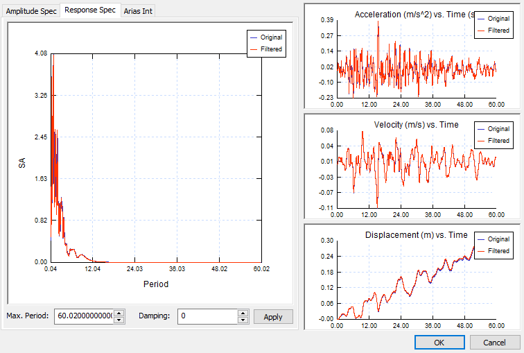
As shown in the figure above, the dialog is made up of three panels. The panel on the left displays the raw time history data and contains controls for various filtering options. The middle panel displays Amplitude Spectrum, Response Spectrum, and Arias Intensity graphs and the panel on the right displays Acceleration, Velocity, and Displacement vs. Time graphs.
Data Filtering
Several filtering options are available to make your Dynamic Analysis more efficient. As you apply these, the various graphs displayed in the dialog are dynamically updated to show both the original and filtered data for easy comparison.
One filtering option is the display of spectrum data for a given frequency range by entering a minimum and maximum in the Filter Spectrum tab. For example, if you observe in the Amplitude Spectrum graph that Amplitude is very minimal for frequencies larger than 10, you can set the maximum frequency to 10.
Another option is filtering data by maximum acceleration response to the load by adjusting the Maximum Period and Damping ratio at the bottom of the Response Spectrum graph.
Filtering all data by Dynamic Load Type by selecting Acceleration, Displacement, or Velocity from the Input dropdown is also an option in the left panel. Finally, you can additionally filter the Amplitude Spectrum by selecting a load type from the dropdown beneath the graph.
Baseline Correction
A part of these powerful filtering options is the ability to apply Baseline Correction in order to correct velocity and/or displacement drift. The option has two methods: Cut Off and Sinusoid. Once either Velocity or Displacement is corrected, new sets of Acceleration and Velocity or Acceleration and Displacement are calculated based on the corrected values and plotted on the graphs to compare with the original dataset.
Assigning a Dynamic Load Function to a Dynamic Load
Once a Dynamic Load Function is defined and saved, you can assign it to any Displacement, Acceleration, or Velocity Dynamic Load using the Define Dynamic Loads dialog. (Dynamic > Define Dynamic Loads). Clicking the X or Y Define button opens the Define Data dialog.
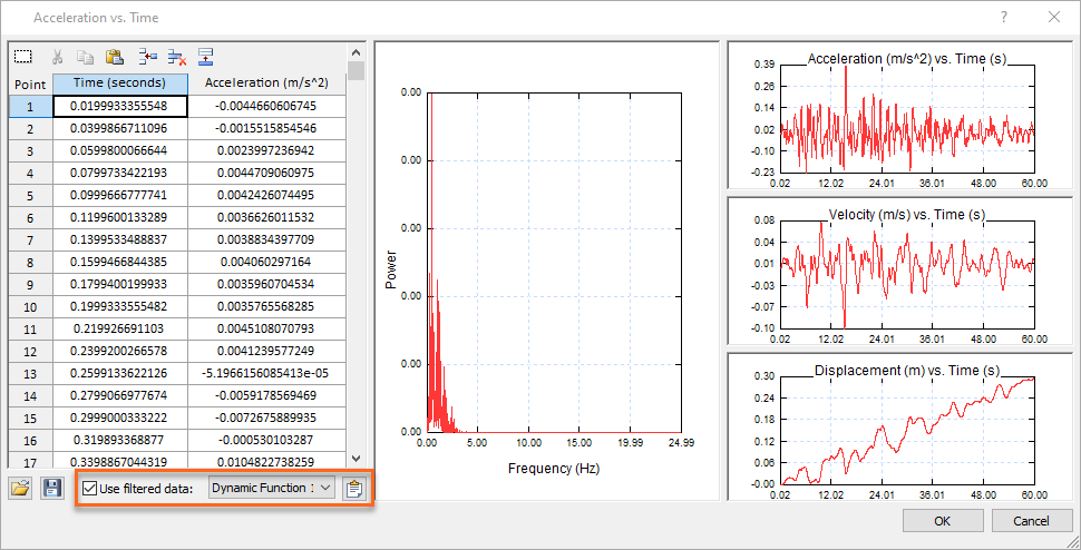
To apply the filtered data, simply select the Use Filtered Data checkbox at the bottom left of the dialog and then select the Dynamic Load Function from the dropdown to the right. To view and further filter the data, click the Filter Data button to the right of the dropdown. This opens the Dynamic Data Analysis dialog where you can analyze and filter the data as discussed above.
Dynamic Pore Pressure Analysis in RS2
RS2 now also has the Finn material model to enable more accurate computation of excess pore pressure generated by a seismic dynamic load. By applying the model to the analysis of a liquefiable material, you can better predict the increase of pore pressure and decrease of effective stress under the action of an external seismic load.
To enable this feature, select the Finn model as the material’s Strength Failure Criterion, then set the material’s Hydraulic Properties to Undrained. When Undrained is selected, you can manually input the Fluid Bulk Modulus to increase the numerical stability of your analysis.
New Dynamic Boundary Conditions in RS2
Rounding out the roster of great new RS2 features is the addition of two new Dynamic Boundary Condition types: Hydro Mass and Nodal Mass. These options dramatically increase the power and flexibility of RS2’s Dynamic Analysis of dams and embankments.
The Hydro Mass option provides flexibility in RS2 to account for cases where the material is dry, but water is acting on its surroundings, such as a concrete dam. When selecting this boundary condition, you can manually enter pore pressure input as the height of the water in the reservoir as well as the base elevation of the reservoir.
The Nodal Mass option has bi-directional input and allows you to assign an additional mass to a node to simulate the dynamic load from an external force.
New Shear Strength Reduction Graph in RS3
Adding to the already powerful and comprehensive array of results graphs in RS3 is the ability to plot the relationship between Shear Strength Reduction and Maximum Total Displacement when conducting a Shear Strength Reduction analysis. To generate the graph, simply select Shear Strength Reduction on the Graph menu.
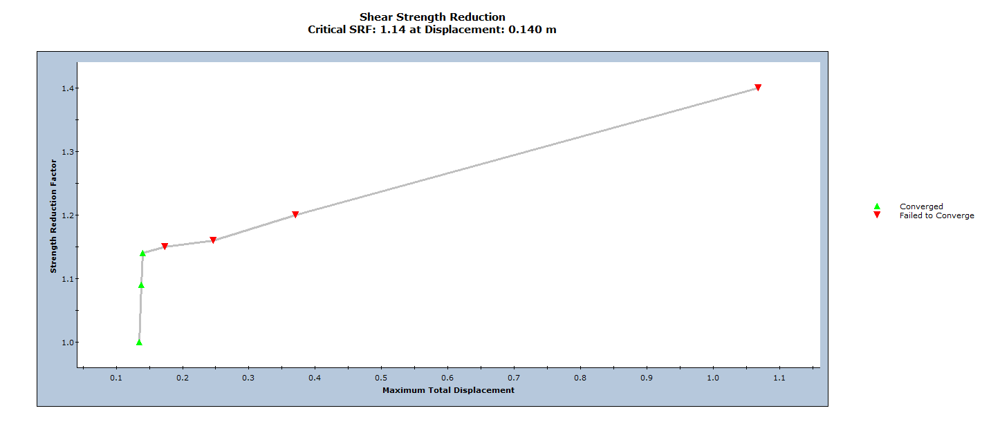
Some of the highlights of this new graphing capability are:
- Each data point represents the Shear Strength Reduction Factor versus the Maximum Displacement for one iteration of the SSR analysis. The Maximum Displacement is the maximum value of Total Displacement that occurred at any point in the model, for the stress analysis that was computed using that value of Strength Reduction Factor.
- Data points displayed in green represent analyses for which the stress analysis results achieved convergence within the specified tolerance for the analysis. The tolerance is the Tolerance (SRF) value in the Strength Reduction tab of the Project Settings dialog.
- Data points displayed in red represent analyses for which the stress analysis did NOT achieve convergence within the specified tolerance (i.e., the model was unstable).
- The Critical Strength Reduction Factor (Critical SRF) is the maximum value of SRF for which the model remains stable (i.e., the analysis converges). This is the uppermost green data point on the graph.