Using Rocscience Tools to Implement Deep Foundation Resistance While Performing Slope Stability Analysis
- Sina Javankhoshdel, Senior Manager - LEM at Rocscience
Deep Foundations Institute recently hosted the virtual conference S3: Slope, Slides, and Stabilization on August 5th, 2020, and the Rocscience Team was represented by Dr. Sina Javankhoshdel and Jeff Lam in the software discussion panel as part of the event. This gave us the opportunity to highlight the features and showcase the application of our software programs to a specific slope stability analysis problem, with the goal of advancing the state of practice.
This year’s discussion was focused on the correct implementation of deep foundation resistance in slope stability analysis. As will be seen, Rocscience took a novel approach to the problem by using five of its software programs - Slide2, RSPile, RS2, Slide3, and RS3 with Slide2 serving as the fulcrum for other analyses beyond the commonly used 2D limit equilibrium. This follows on the best practice of verifying results using a different analysis method (limit equilibrium vs. finite element) as well as comparing 2D results with a 3D analysis to determine the significance of 3D effects. It also showcases how these Rocscience programs can be used in cooperation with each other for a comprehensive and realistic analysis result.
The Problem
The Trunk Highway in Crookstone, Minnesota was the subject of this year’s discussion, where a landslide took place on a slope in 2003; the same location that was subject to a landslide that took place 70 years before in 1933. This landslide history is prominent in the baseline conditions defined in the problem that addresses the common practice of applying the full shear strength of the structural material as a resisting force whereas reality is that the deep foundation element often reaches a different failure mode before mobilization of its full shear strength
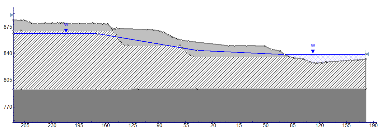
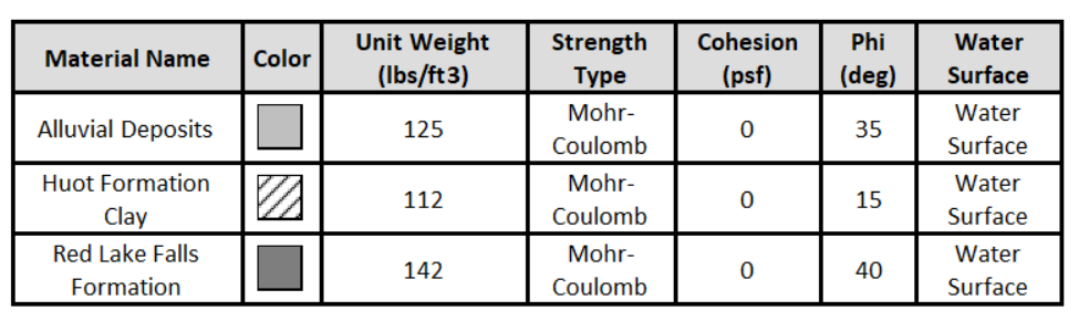
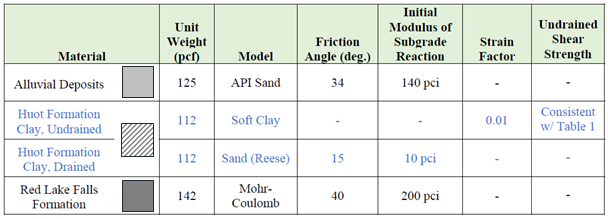
A snapshot of the provided model is shown in Figure 1 while Table 1 below shows the material properties for the baseline analysis.
For the baseline problem, the goal is to analyze the slope, including stabilization, using three rows of 8.0-ft diameter drilled shafts, as shown in Figure 2.
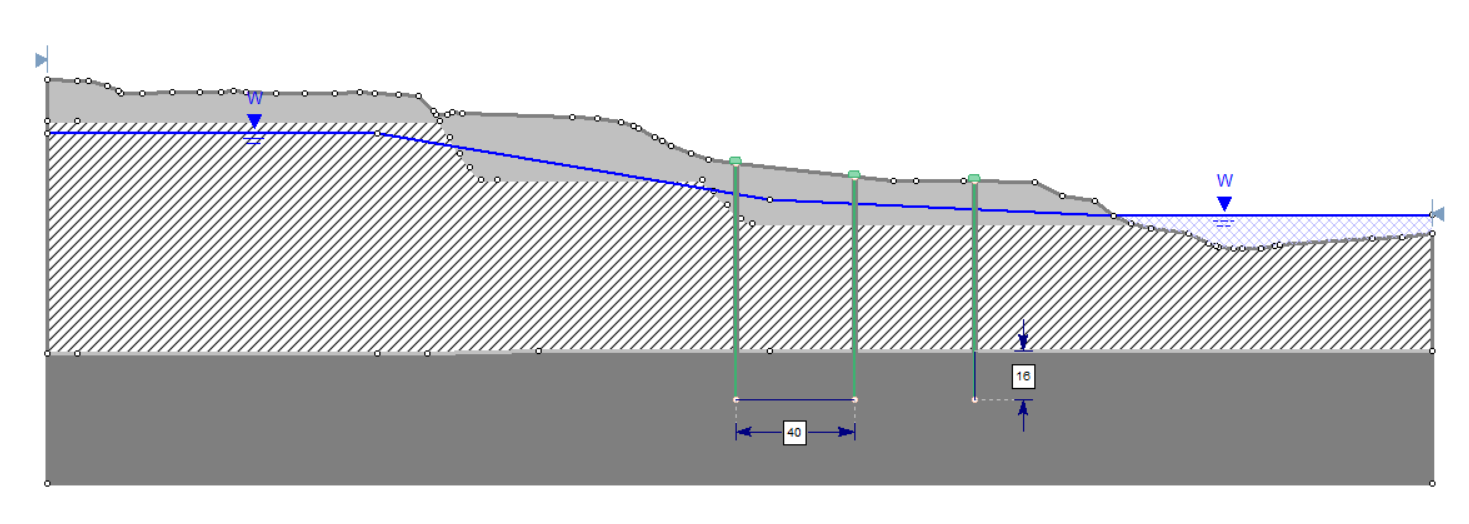
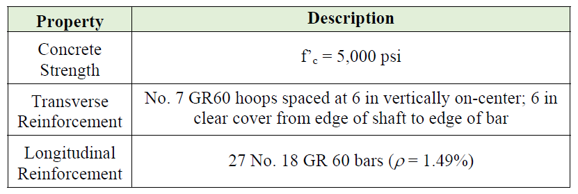
The provided model also identifies the location of the drilled shafts, which are spaced at 40 ft apart in the plane of the cross-section and 24 ft in the out-of-plane direction. The shafts are socketed 16 ft into the Red Lake Falls Formation, meaning that the length of each row is slightly different because of changing ground surface elevations. Table 2 below gives additional structural properties of the drilled shafts, while Table 3 provides the recommended parameters for defining p-y curves for the lateral pile analysis.
Analysis and Results
Rocscience has taken a six-step approach to the problem where five Rocscience software programs are used interoperably for a comprehensive and detailed analysis:
Step 1. Using Slide2 to determine the FoS for existing conditions of the baseline problem for a 2D limit equilibrium analysis
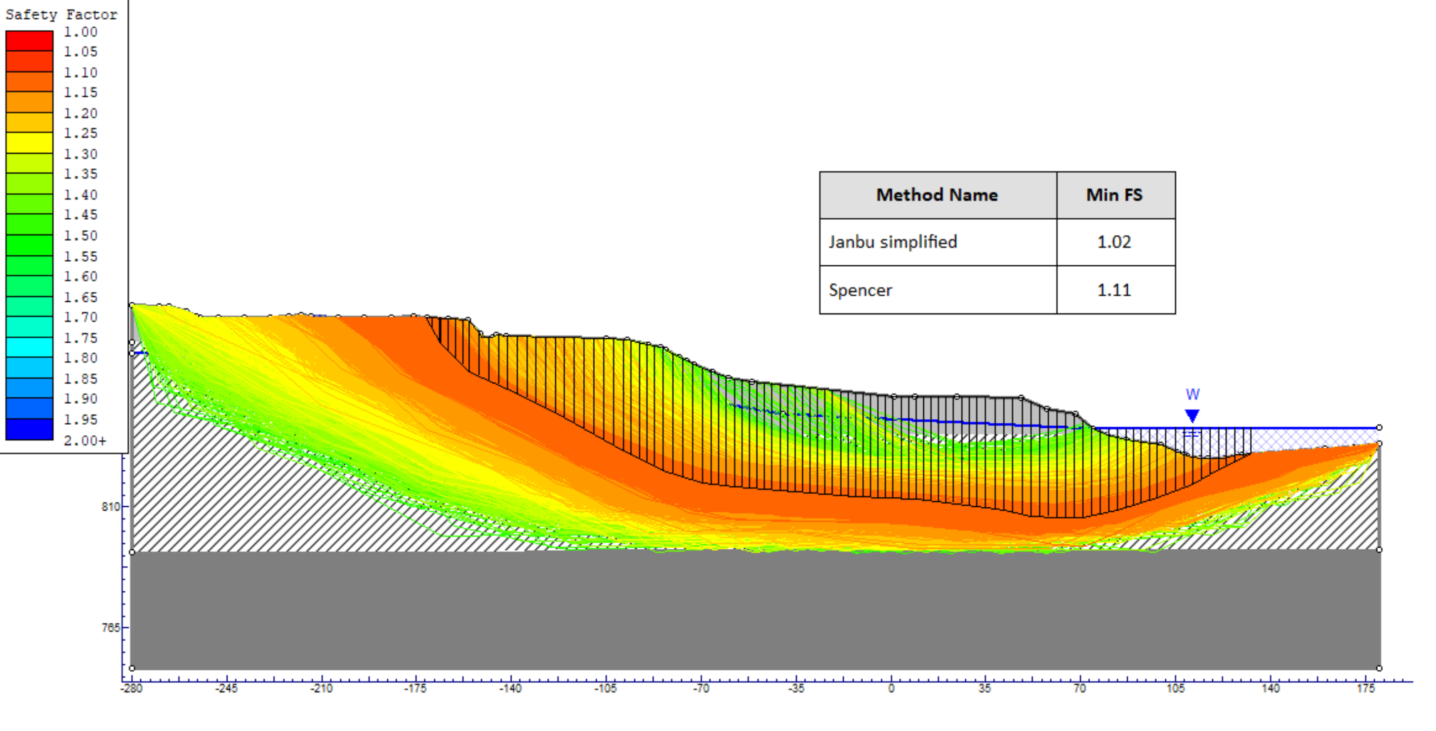
As the starting point for the problem solution, the provided baseline model (Figure 1) is imported into Slide2 using its powerful geometry import and cleanup capabilities. The material properties are then defined for the model, as shown in Table 1. A non-circular critical slip surface search is then conducted to determine the FoS of the baseline model using Cuckoo Search coupled with Surface Altering Optimization (SAO). SAO is a powerful tool unique to Rocscience programs that yield lower FoSs by modifying the geometry of a given slip surface. The resulting FoS (using the Spencer method) is 1.11, as shown in Figure 3.
Step 2 – Using RSPile to determine the allowable soil displacement that will produce the nominal drilled shaft structural mobilization
In this step, the Slide2 model is first set up with reinforcing elements as shown in the provided drilled shaft design (see Figure 2). A lateral analysis is then set up in RSPile using the provided drilled shaft structural properties (Table 2) and p-y parameters (Table 3).
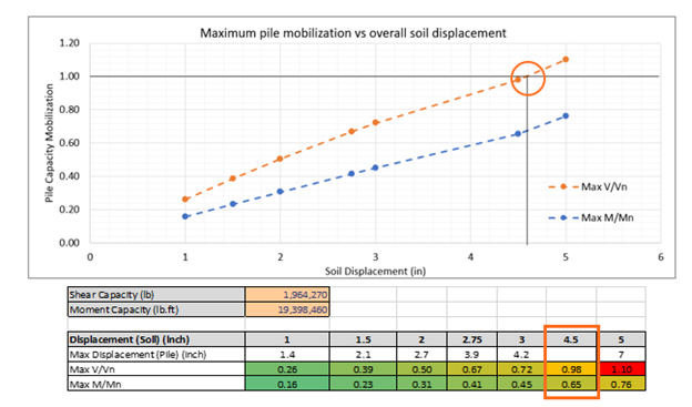
The structural mobilization along the pile length vs. a range of soil displacements is then checked to see how much deformation the pile can handle. Figure 4 below shows the structural mobilization of the pile at a 1” displacement while Figure 5 shows the maximum pile mobilization vs. a range of soil displacements.
Step 3 – Using Slide2 and RSPile to determine the FoS of the reinforced slope
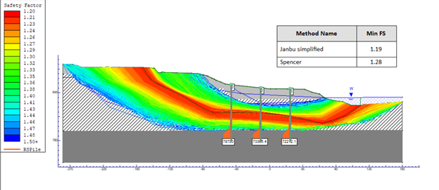
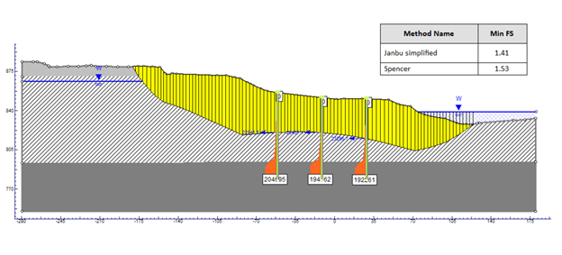
Once the pile’s structural mobilization is calculated, the RSPile files are linked into Slide2 for the slope stability analysis using Slide2’s automated integration with RSPile. Once the files are linked, the pile resistance envelope for each pile stratigraphy is generated and used by the searching algorithm in Slide2 to determine the critical sliding surface. At a soil displacement of 1” (Figure 6), the FoS is 1.3. If this is the target FoS, it is the geotechnical stability of the system that governs since there is still structural capacity left in the piles. To see what it takes to get a FoS of 1.5, the soil is allowed to continue to displace up to 2.75”, as shown in Figure 7.
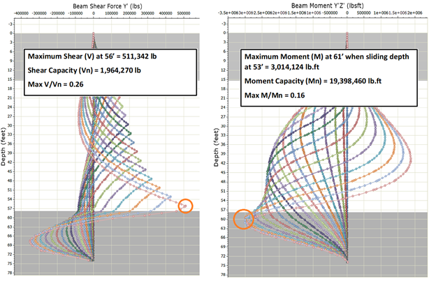
The analysis is then taken further by running additional analyses in RSPile to see how the pile will perform as displacement along the critical sliding depth is increased until hitting full structural mobilization (Figure 8).
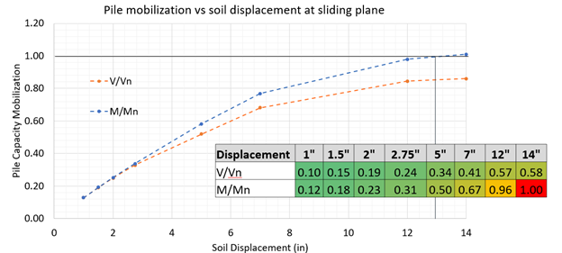
The conclusion from the results is that the flexural capacity of the pile will be reached first when only 58% of the nominal shear capacity is mobilized.
Step 4 – Using RS2's SSR capability to analyze FoS of the Slope
Since best practice dictates that results are checked using a different analysis method, a comparable finite element analysis is conducted for comparison purposes. Model materials are imported as MC, and a plastic model is used for the soils where the residual strength is equal to peak strength. Pile parameters of E and Moment of Inertia are calculated from the provided pile parameters (Table 2 and Table 3), and the pile is modeled as a simple liner with no slip.
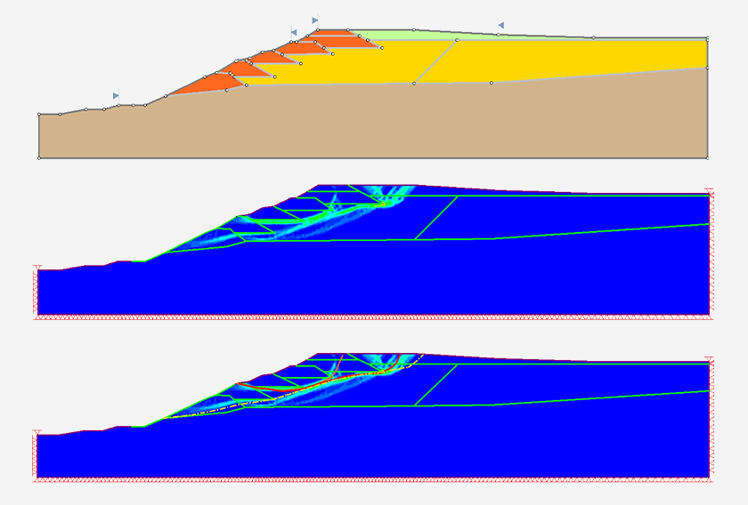
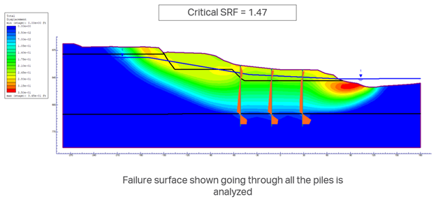
The first step in the analysis is to compare the unreinforced case to ensure that a) a comparable FoS and b) a comparable critical surface are obtained. The reinforced model is then analyzed with a failure surface going through all the piles to produce a strength reduction factor (SRF) of close to 1.5, which is similar to our 2D limit equilibrium results (Figure 9).
RS2 automatically generates the steps to calculate the strength reduction factor (SRF) with an SRF and indicates whether the pile (liner) has reached its structural capacity. The results are presented in the table in Figure 10 and Figure 11 below, with the results being in agreement with the RSPile model that the pile is mobilizing more moment as the soil continues to deform.
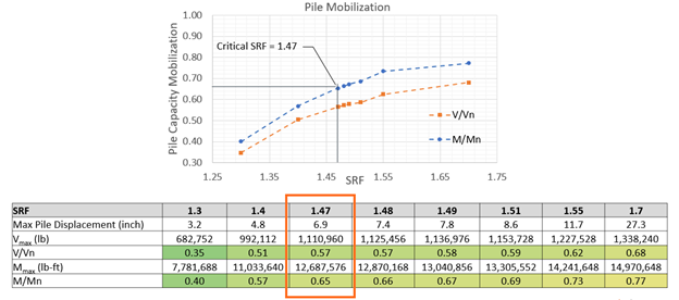
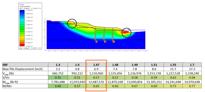
It is also shown in the figures that, at our critical SRF of 1.47, the geotechnical stability of the soil governs.
Step 5 – Using Slide3 to determine the significance of 3D effects with a 3D limit equilibrium analysis
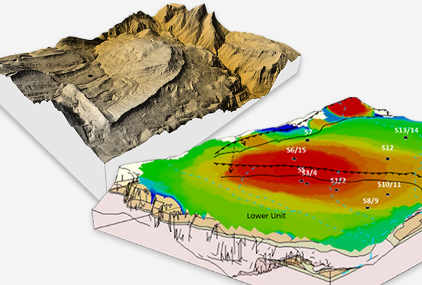
To perform a proper analysis of the influence of support (piles) on the slope stability, full 3D models of the problem were created in Slide3 to compare with the 2D results. The models were created using the provided elevation contours together with the boreholes to create a second geometry, which was more accurate since actual elevation contours were used.
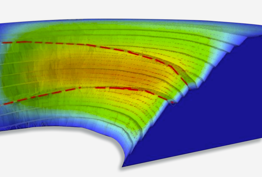
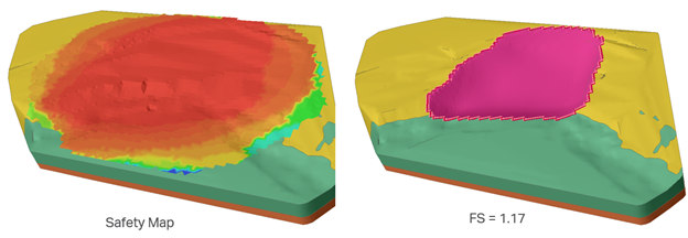
The results of the unreinforced 3D limit equilibrium analysis can be seen in Figure 12.
Step 6 – Using RS3 to compare the results obtained from the Slide3 analysis
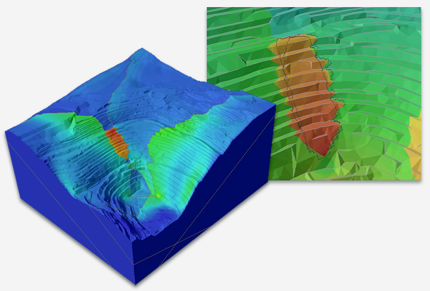
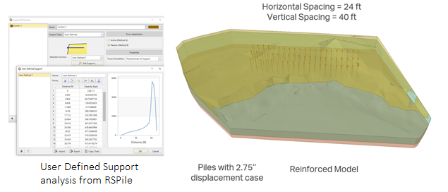
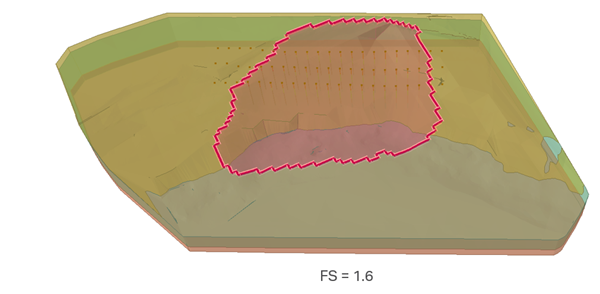
The next and final step in the problem solution is to take geometry from Slide3 into RS3 for comparison with the 3D limit equilibrium analysis. To create the reinforced model, the capacity and the piles for the 2.7” displacement are exported as user-defined supports. The pattern is similar to the 2D, H-spacing of 24 ft, and V-spacing of 40 ft for the region. The analysis is first performed for the reinforced case, obtaining a FoS of 1.6, which is slightly higher than the 2D reinforced case, which is as expected. The model and results are presented in Figure 13 and Figure 14 below.
Summary of Results
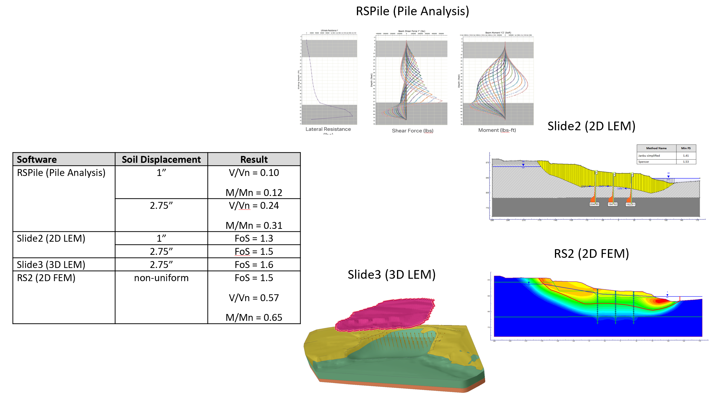
To summarize the results of the analyses:
- Slide2 yielded two different FoS based on soil displacement.
- A strength reduction factor (SRF) of close to 1.5, which is similar to our 2D limit equilibrium results was achieved when the Slide2 results were verified using RS2.
- The result of the analysis in Slide3 was verified with that of RS3 with the FoS being 1.6.
Conclusion and Takeaway
Rocscience has taken a broad approach to the problem by using five of its software programs (Slide2, RSPile, RS2, Slide3, and RS3) in collaboration. Slide2 was chosen to serve as the fulcrum for other analysis methods due to the general popularity and widespread acceptance of the 2D limit equilibrium method. The results from the analysis indicate that 2D LEM (Slide2) combined with pile analysis software (RSPile) will yield comparable results when compared to other more sophisticated methods such as 2D FEM (RS2), as long as the material parameters are comparable and the failure mechanisms are modeled correctly. For example, all analysis models correctly indicate that the piles will mobilize its full flexural capacity before shear occurs along with the critical sliding surface, and it is the flexural capacity that governs over the range of soil displacements analyzed,
A comparison of 2D and 3D results indicate a marginal increase (6%) in FoS when the problem is analyzed in 3D. The difference is due to the limitations of a 2D model, which incorrectly assumes a plane strain failure surface, and neglects confinement forces.
For the analysis of the subject pile reinforced slope, the engineer can choose from multiple analysis methods to compute the FoS. The decision of which method to use would ultimately depend on the amount of soil strength data available, resolution of topographic data, budget, time, and the engineer’s experience with the corresponding method.