On the comparison of 2D and 3D stability analyses of an anisotropic slope
The Adoption of 3D Limit Equilibrium Method
2D limit equilibrium analysis is a powerful tool for problems involving uniform geometry. Three-dimensional limit equilibrium modeling can be an excellent method for problems with more complex geometry as it considers the normal and horizontal side resisting forces along the sides of the sliding mass. It is also becoming more widely available for commercial use and more user friendly, allowing geotechnical engineers to better assess a slope’s stability in more detail.
Parametric Study of an Open Pit Mine
This paper summarizes the results of a parametric study using 2D and 3D LEM to demonstrate the variability in Factor of Safety (FOS) for a highly bedded open pit mine. This example uses an Iron ore mine located in the Pilbara region of Western Australia.
Slide2 and Slide3 were used to calculate the factor of safety of the slope. Slide2 uses the method of slices while Slide3 uses the method of columns, to find the force acting on the failure surface (i.e. mobilized stress) and these are compared to the available shear strength to evaluate the factor of safety.
To find the difference in FOS using 2D and 3D limit equilibrium methods, a series of models were computed with the following variables.
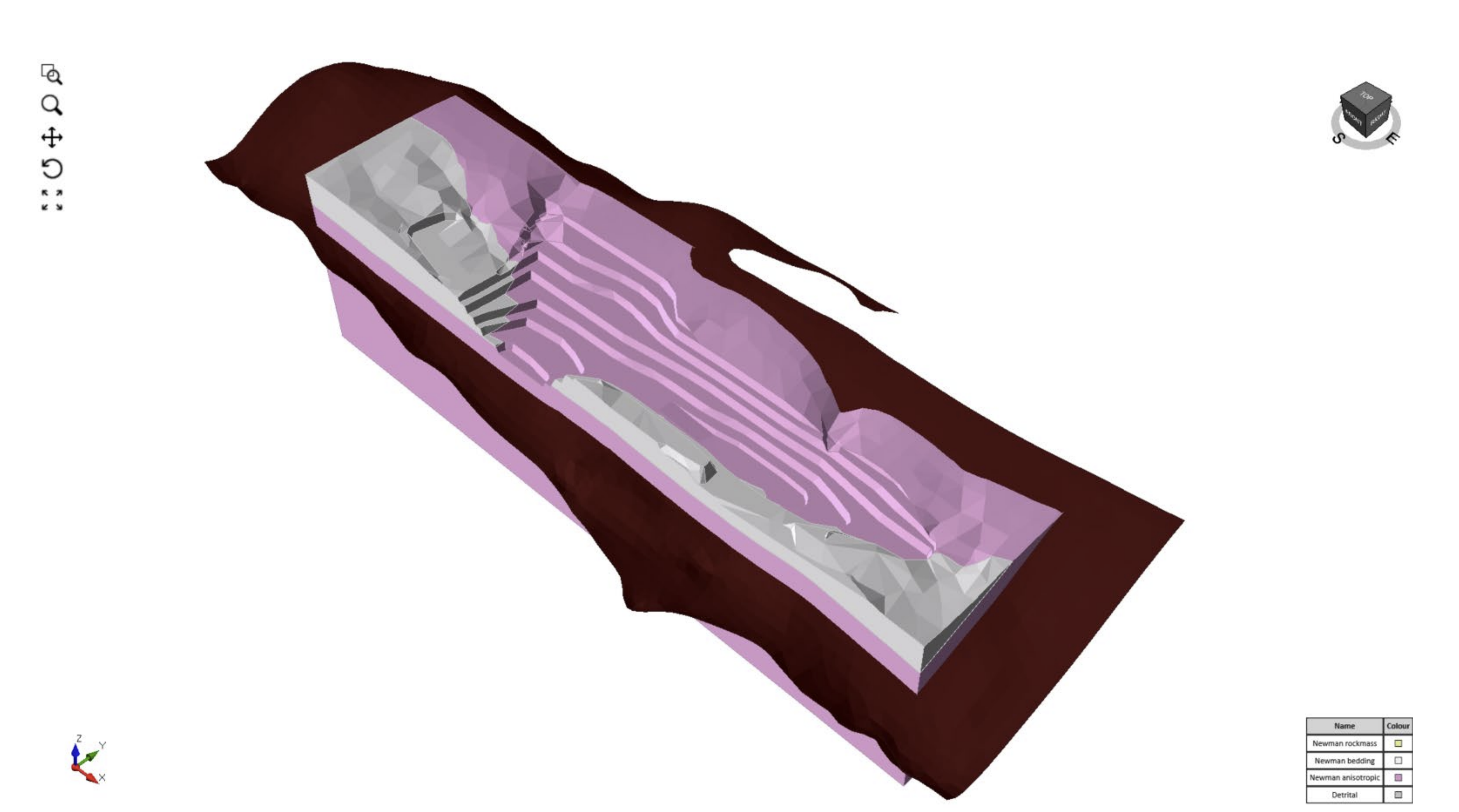
- 3D models using the mine design, natural surface topography and lithological surfaces exported from the geological model (Figure 1). The deposit was above the water table, so pore pressures were not considered. Anisotropy and true dip are included in 3D LE models;
- 2D models using a 2D section cut through the middle of the critical slip surface calculated from 3D modelling (Figure 2). Apparent dip is inherently included in 2D LE models;
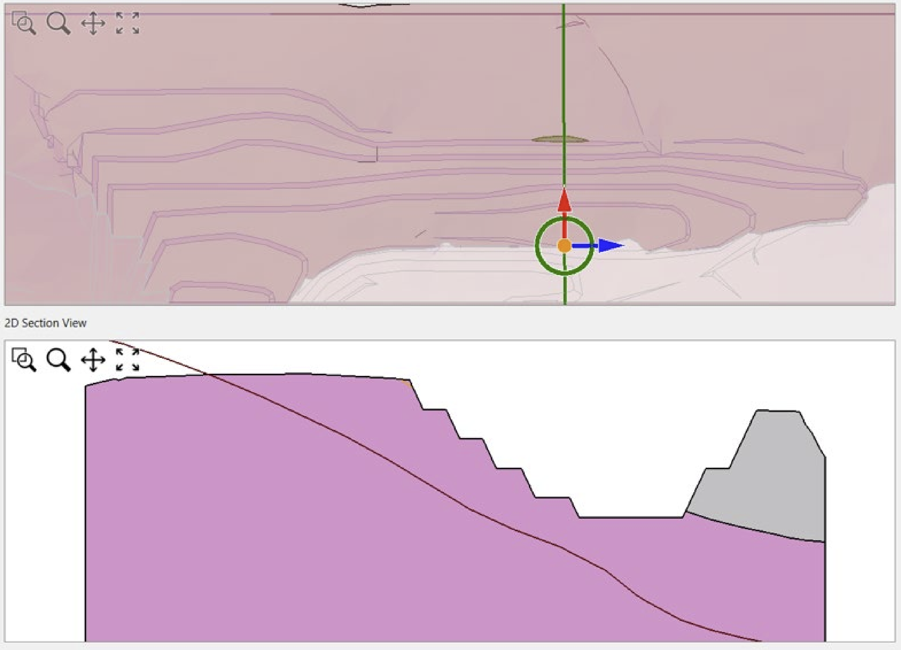
Figure 2 Plan view map showing location and cross-section cut for Slide2 analysis from the Slide3 model - 3D models derived by extruding the 2D section at varying lateral slope lengths (50 m, 100 m, 150 m, 200 m, 400 m). True anisotropy is not included in 2D extruded models. Instead, the third dimension is added by uniform extrusion of a 2D section.
- Cuckoo vs Particle Swarm slip surface search methods, at varying search options (i.e. number of search surfaces and search depth limits); and
- Linear (i.e. Mohr-Coulomb) and Non-Linear (Shear-Normal, Generalized Hoek-Brown and Barton-Bandis) material strengths.
Results
Through this analysis, the following results were found about the performance of both the 2D and 3D methods.
For the full 3D analysis (Table 1), the results showed that when using nonlinear strength criteria, a lower factor of safety was calculated compared to linear strength models. The full 3D analysis also showed that the application of search depth limits generally results in a higher factor of safety when compared with no search depth limits being applied. The results of FOS vary from 0.81 to 1.14.
Dimension |
Material Model |
Search Method |
Number of Nests / Particles |
Slope Depth Limit |
Critical FOSGLE |
Reference Figure |
3D |
Non-Linear (GHB + BB) |
Cuckoo |
20 |
None |
0.90 |
Figure 4 A |
Cuckoo |
80 |
0.89 |
Figure 4 B |
|||
Particle Swarm |
20 |
0.90 |
Figure 4 C |
|||
Particle Swarm |
80 |
0.81 |
Figure 4 D |
|||
3D |
Non-Linear (GHB + BB) |
Cuckoo |
20 |
15m |
1.13 |
Figure 5 A |
Cuckoo |
80 |
1.00 |
Figure 5 B |
|||
Particle Swarm |
20 |
1.08 |
Figure 5 C |
|||
Particle Swarm |
80 |
1.06 |
Figure 5 D |
|||
3D |
Linear (MC) |
Cuckoo |
20 |
None |
1.10 |
Figure 6 A |
Cuckoo |
80 |
1.11 |
Figure 6 B |
|||
Particle Swarm |
20 |
1.06 |
Figure 6 C |
|||
Particle Swarm |
80 |
1.11 |
Figure 6 D |
|||
3D |
Linear (MC) |
Cuckoo |
20 |
15m |
1.12 |
Figure 7 A |
Cuckoo |
80 |
1.10 |
Figure 7 B |
|||
Particle Swarm |
20 |
1.14 |
Figure 7 C |
|||
Particle Swarm |
80 |
1.09 |
Figure 7 D |
Table 1 Parametric study results – 3D LE analysis. Reference Figure’s correspond with the original paper figures.
Findings show that the FOS values from the 2D analysis (table 2) were generally lower than the 3D analysis varying from 0.73 to 0.88.
The difference in the factor of safety is also more pronounced when linear models are applied. This is because the rock mass strength at the sides of the failure surface is not considered in the 2D analysis but is included in the 3D analysis due to the 3D shape of the slip surface.
Dimension |
Material Model |
Search Method |
Slope Depth Limit |
Critical FOS GLE |
Reference Figure |
2D |
Non-linear (GHB + BB) |
Cuckoo |
None |
0.73 |
Figure 8 A |
Particle Swarm |
0.84 |
Figure 8 B |
|||
Linear (MC) |
Cuckoo |
0.84 |
Figure 8 C |
||
Particle Swarm |
0.88 |
Figure 8 D |
|||
3D |
Non-linear (GHB + BB) |
Cuckoo |
15 m |
0.80 |
Figure 9 A |
Particle Swarm |
0.80 |
Figure 9 B |
|||
Linear (MC) |
Cuckoo |
0.85 |
Figure 9 C |
||
Particle Swarm |
0.85 |
Figure 9 D |
Table 2 – Parametric Study Results – 2D LE analyses. Reference Figure’s correspond with the original paper figures.
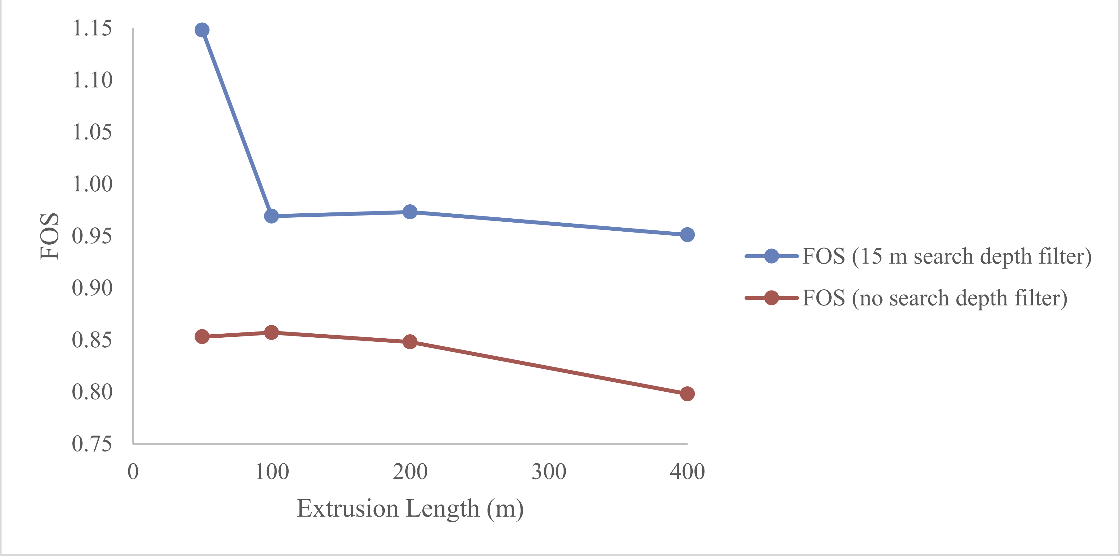
The results from the extruded models also show that length of extrusion of the 2D sections will affect the factor of safety. The factor of safety will be higher when the extrusion length is smaller and thus the slope is more confined (Figure 3).
How can this help you with your projects?
This paper highlights the variance in FOS between 2D and 3D LE methods and that 3D LEM analysis consistently produces a higher FOS for anisotropic rock masses by capturing a more realistic representation of the slip surface.
3D LE is becoming widely adopted for complex engineering problems by giving you a better representation of your problem.