Latest Features in RS2
RS2 is a dynamic 2D Finite Element Analysis program designed to help you overcome your most challenging geotechnical problems. RS2 can be used for a variety of applications including embankments, mining, tunneling, foundations and more.
Stay up to date with the latest features and integrations that you can incorporate into your geotechnical projects.
August 2022
Thermal Module in RS2
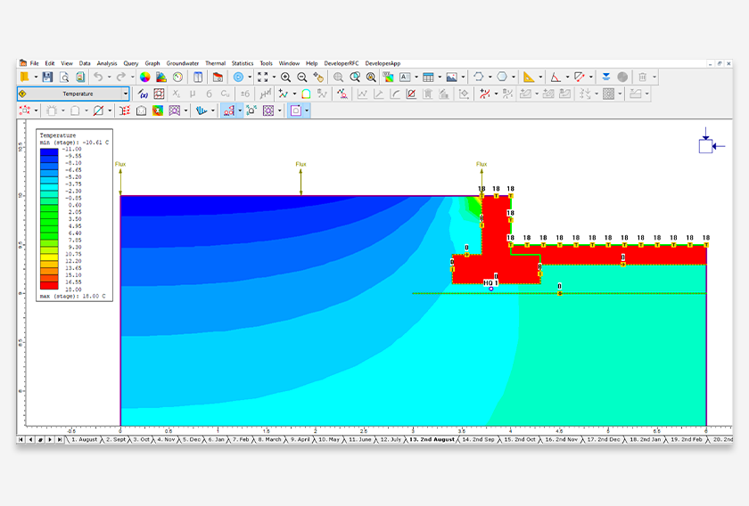
The thermal module in RS2 is a new feature designed to simulate 2D thermal analysis for various geotechnical structure models using finite element methods. Thermal-hydro-mechanical coupling analysis is also supported within this module. In a thermal geometry, static temperature and heat transfer can be modeled, the thermal properties can be defined for liner and solid elements. Various thermal boundary condition types are provided in the program, including conditions with a thermosyphon system, boundaries with insulation, and convective heat transfer conditions. The thermal deformation and stability of a model can be evaluated from the analysis results.
Thermal Module Applications
The thermal module can be used to model various thermal behaviours, such as ground stability using an artificial ground freezing technique, a thermal design for geo-structures using insulation to prevent soil freezing or using thermosyphon to prevent soil thawing, effects of seasonal changes on the regional water flow, effects of temperature changes to the geotechnical design due to thermal expansion/contraction, etc. You can have a look at more examples and verification models with the RS2 thermal analysis.
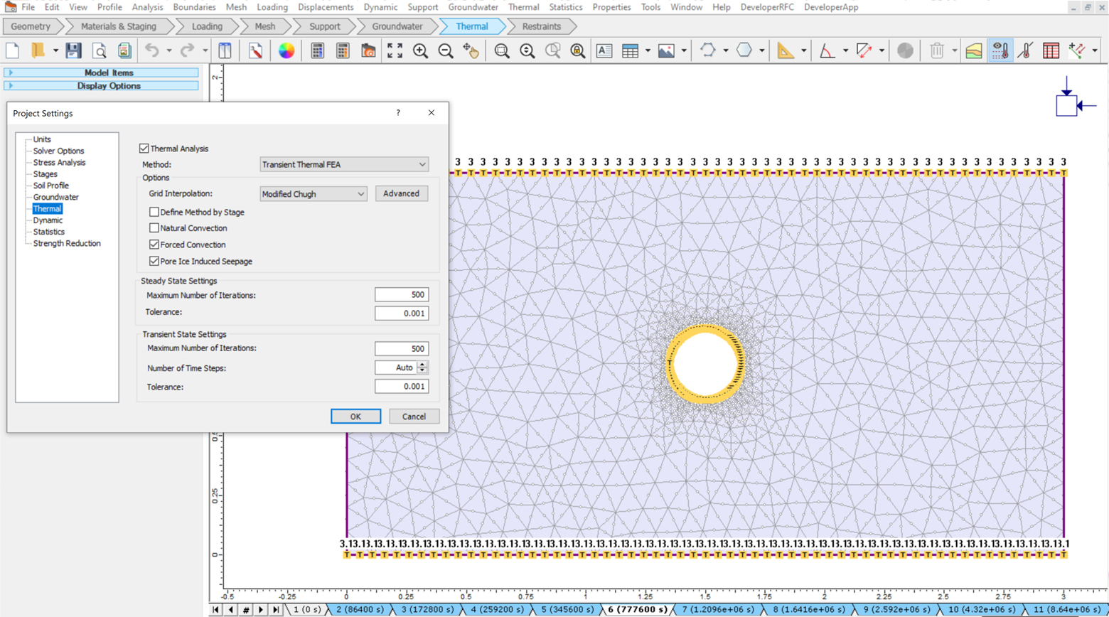
Thermal Methods
Other than static temperature, thermal flow can be modeled using finite element methods, including both steady-state and transient. In addition, natural convection, forced convection, and pore-ice-induced seepage mechanisms are available for thermal-hydro-mechanical coupling analysis. Thermal expansion and thermal dispersivity can also be accounted for.
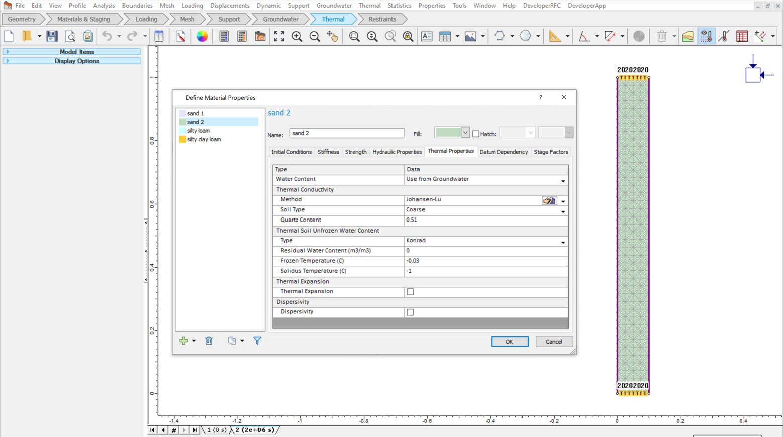
Material Properties
For liner and solid materials, the thermal properties can be defined with different calculation models combined with groundwater setting considerations in RS2. Essential thermal properties include initial temperature condition, water content, thermal conductivity, heat capacity, thermal soil unfrozen water content, thermal expansion, and dispersivity.
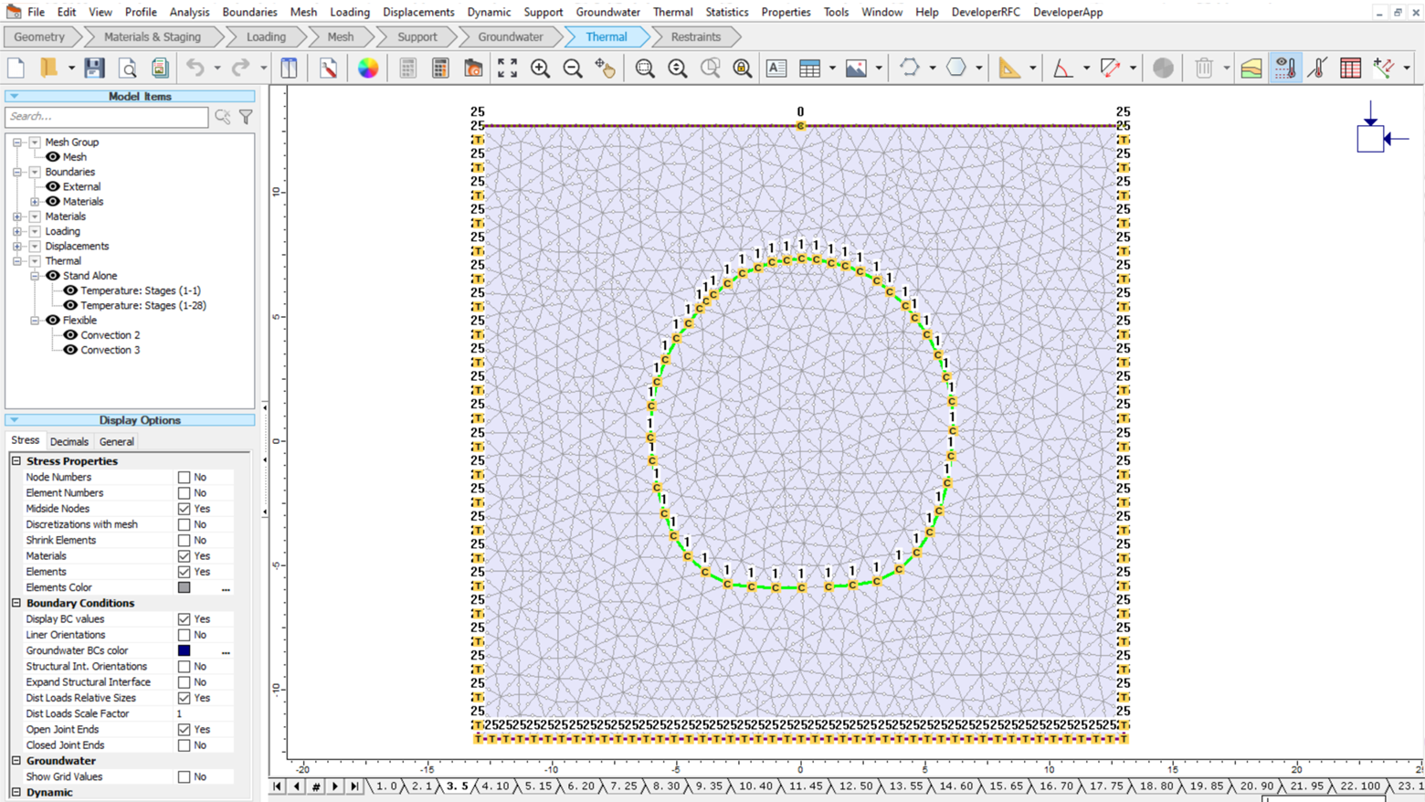
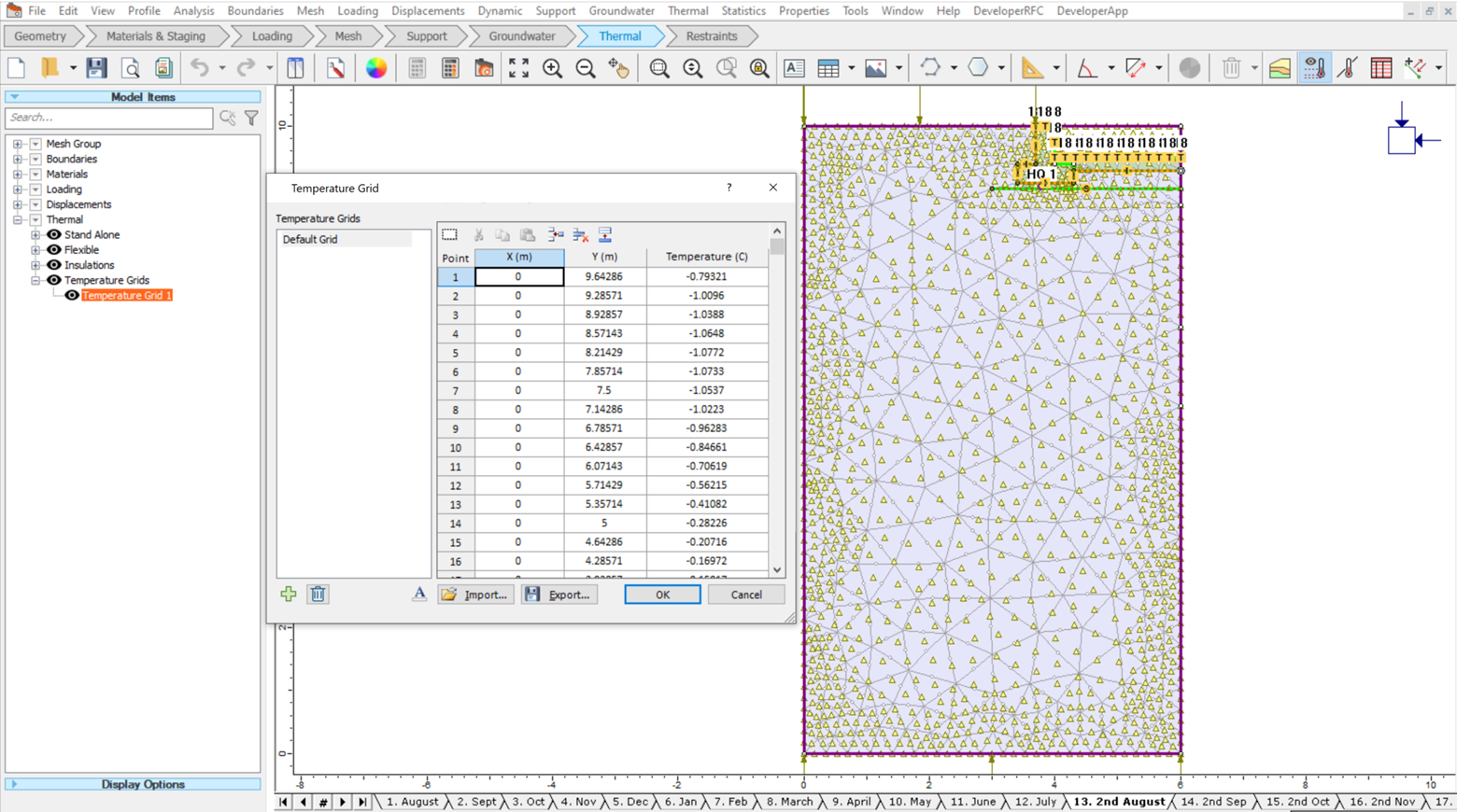
Thermal Geometry Modelling
You can also define the static temperature distribution of the model geometry by inputting grid points with their point temperature. To model heat flow, you can apply a heat transfer section in the model, with a specified heat flow rate.
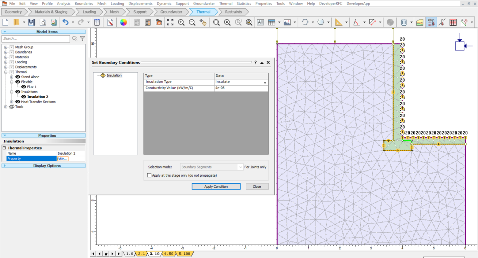
Thermal Boundary Conditions
Thermal boundary conditions are crucial for finite element thermal analysis. RS2 not only allows you to define regular boundary conditions such as temperature, flux, and nodal flux, but can also be used to model more complex cases, such as convection boundary condition to model surfaces exposed to convective heat transfer, thermosyphon boundary condition to model a thermosyphon system, and insulation boundary condition to incorporate thermal conductance between a joint element and the body.
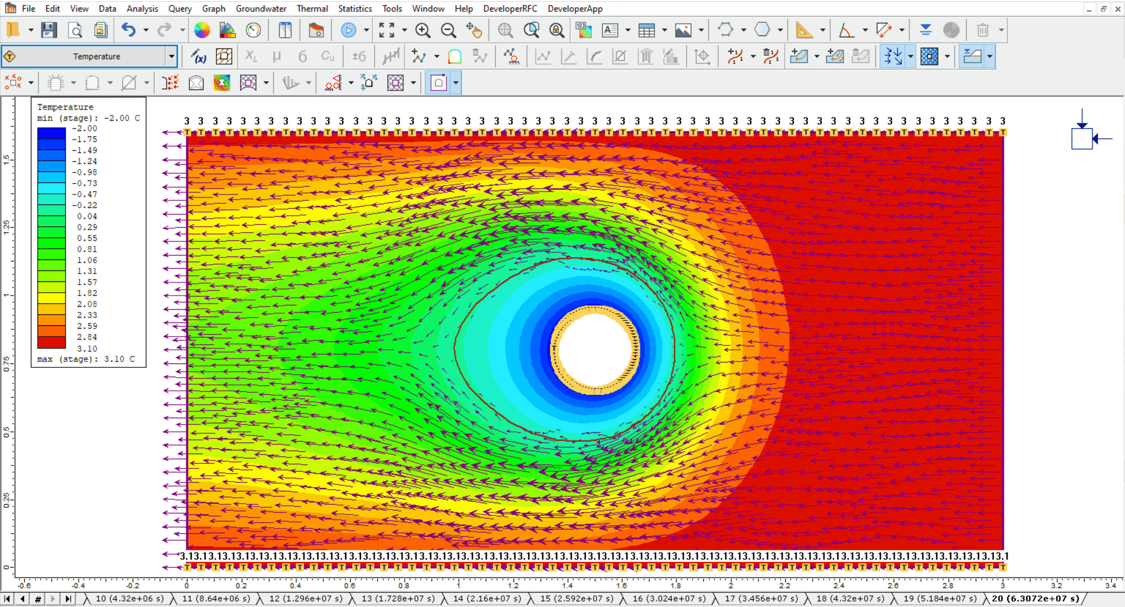
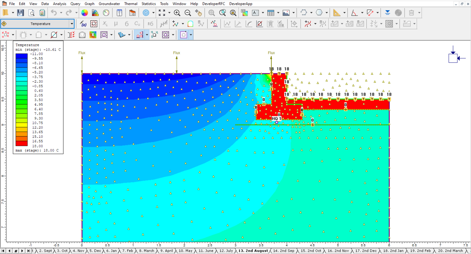
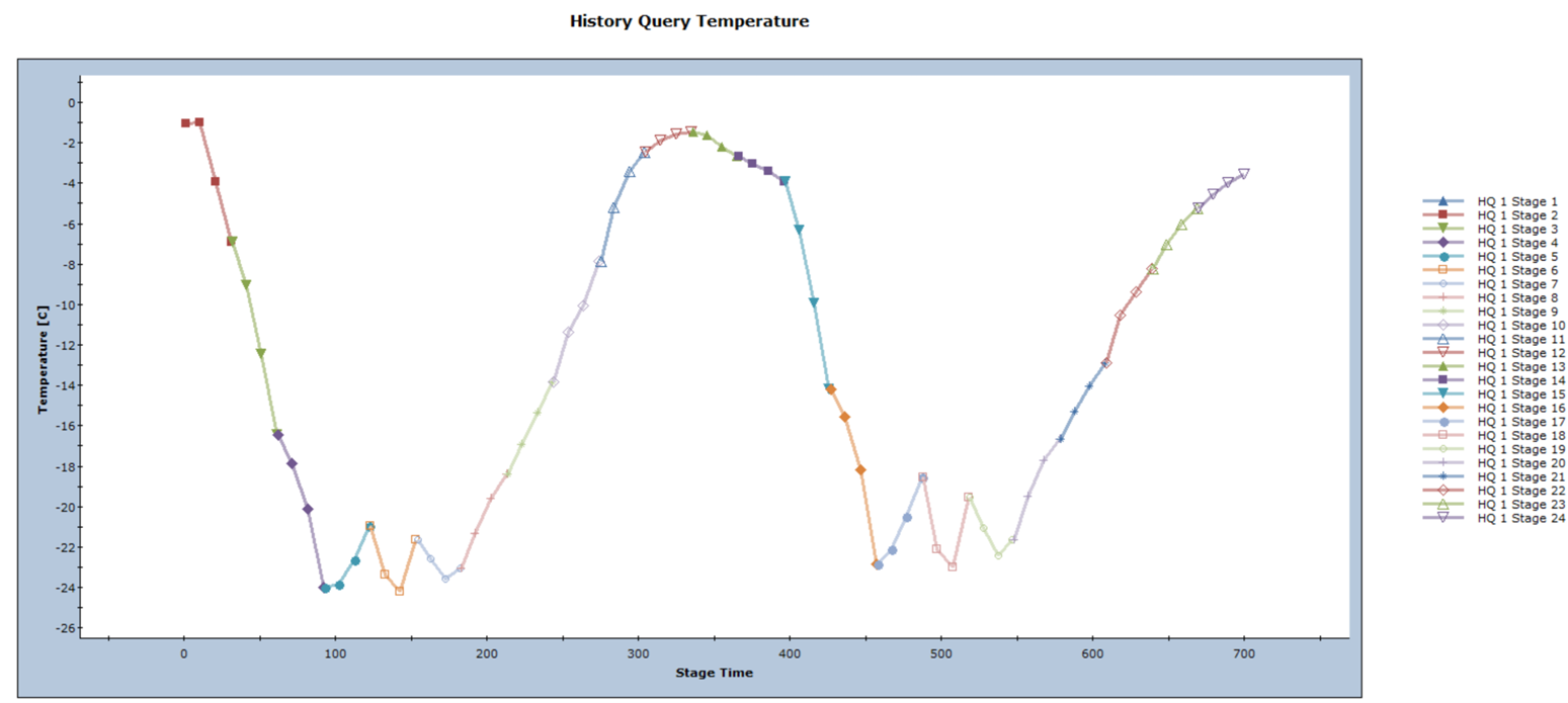
Result Interpretation
The ability to easily visualize and interpret thermal analysis results is important. In RS2, temperature, flux, gradient, conductivity, specific heat, and unfrozen water content can be displayed on the model as contours. To view the historical thermal data of a specific point, graphs of temperature, flux, and gradient over time can be generated. The heat flow directions can also be shown by plotting thermal flow lines.
See the RS2 Thermal Theory Manual for more theories behind the RS2 thermal module. For more thermal model instructions, see the RS2 User Guide.
September 2021
Added Pile Supports in RS2
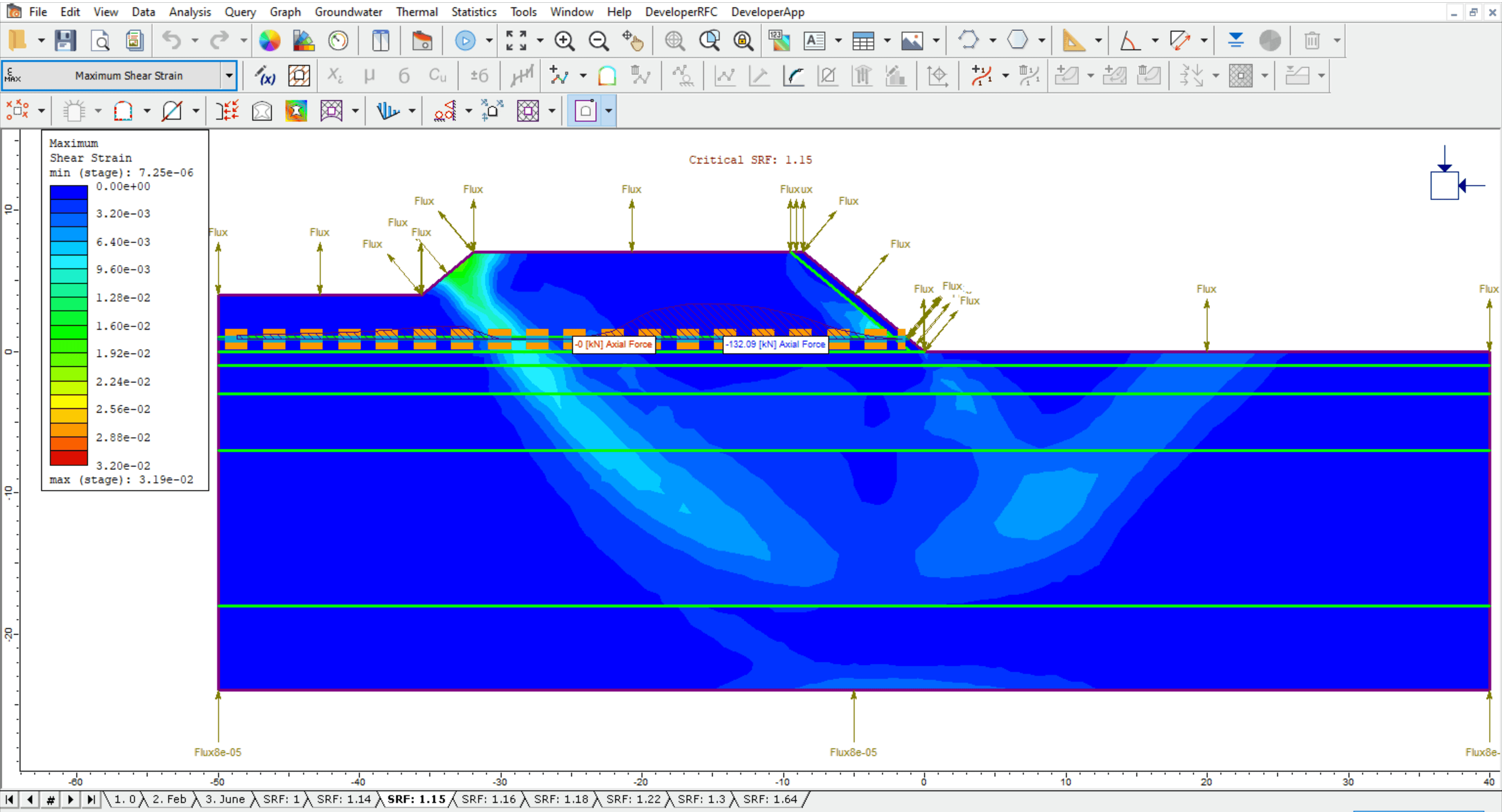
RS2 has improved the ability to model piles using the new dedicated Pile Support Type. Pile supports have a beam component for capturing the structural behaviour as well as an interface component to capture the soil-pile interaction behaviour, namely the skin and end bearing resistance. The new pile support formulation offers improved modelling of soil flow around a pile.
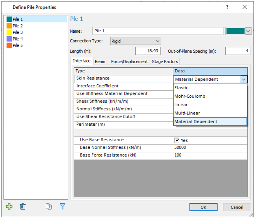
Before this feature was developed, pile behaviour was best captured using structural interfaces which, as the name suggests, also have structural and interface components. Pile properties would need to be converted to equivalent structural interface properties per unit out-of-plane. As shown in Figure 1, with the new dedicated pile support type, the user simply enters the pile properties and out-of-plane spacing. RS2 will take care of the rest. Furthermore, the user can define the pile-to-raft connection type (i.e. free, hinged, rigid, and semi-rigid) which are automatically applied when a pile intersects a liner. The user enters interface properties to define the skin and end bearing resistance. Various skin resistance models are available including Elastic, Mohr-Coulomb, Linear, Multi-linear and Material Dependent.
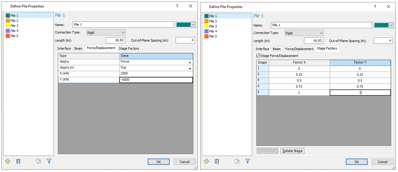
The beam component is defined using the familiar liner properties. The user has the choice of a constant liner property throughout the pile or to define beam segments by length. As shown in Figure 2, the Define Beam segment by length option allows different beam properties along the pile when the design requires multiple sections. As shown in Figure 3, the user can also add forces or displacements on the top or bottom of the pile which can be staged. This can be used for modelling the construction process or pile load tests.
Example: Piled Raft Foundation Design
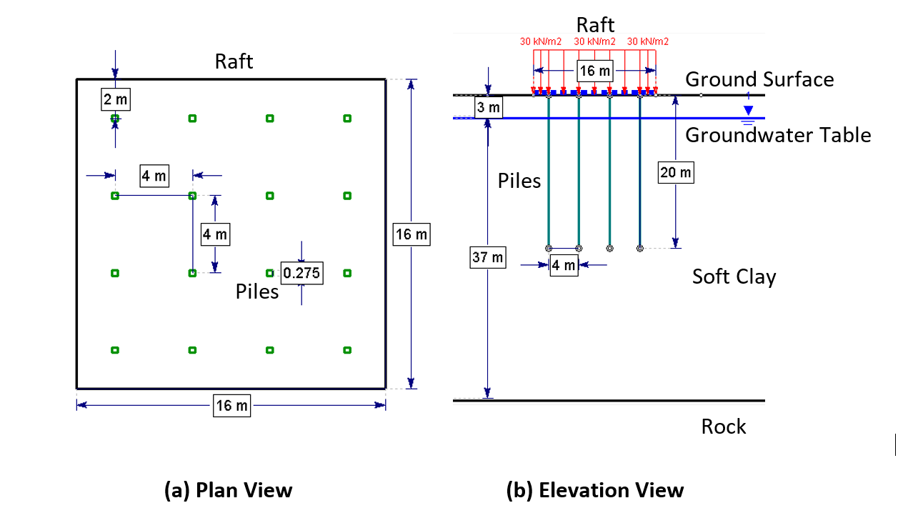
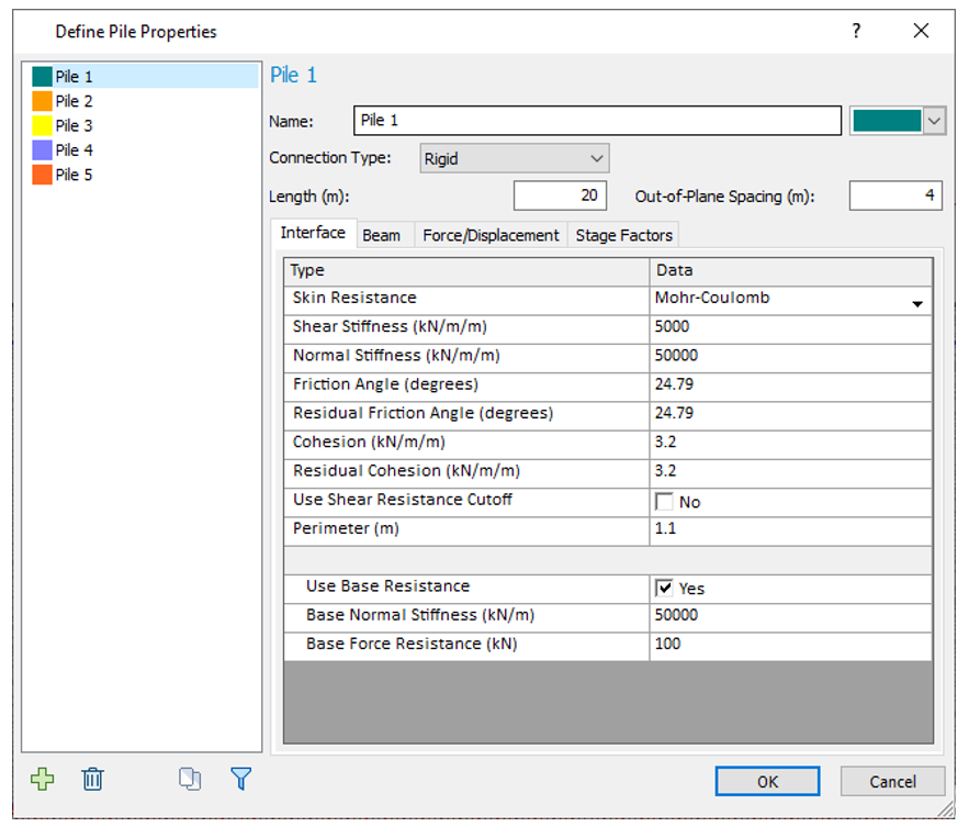
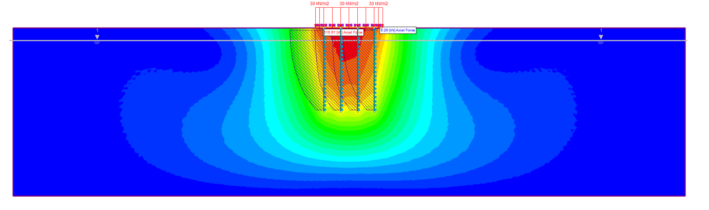
Figure 4 presents a piled raft foundation design. A uniform distributed load of 30 kN/m2 was applied to the piled raft built on a single clay layer. A firm rock layer is located directly under the clay, 40 m from the ground surface. A groundwater table is located 3 m below the ground surface. The 20 m long square pre-cast concrete piles are 275 mm in width and are installed with a 16 x 16 m2 raft. The piles are evenly spaced at 4 m. A Mohr-Coulomb skin resistance model is assumed for the interface behaviour. As shown in Figure 5, the pile properties can be directly entered into the new Define Pile Property dialog. Figure 6 presents the RS2 total displacement contours with pile axial force overlaid to show the performance of the pile raft foundation design. Full details on how to create the model can be found in our Piled Raft Foundation tutorial.
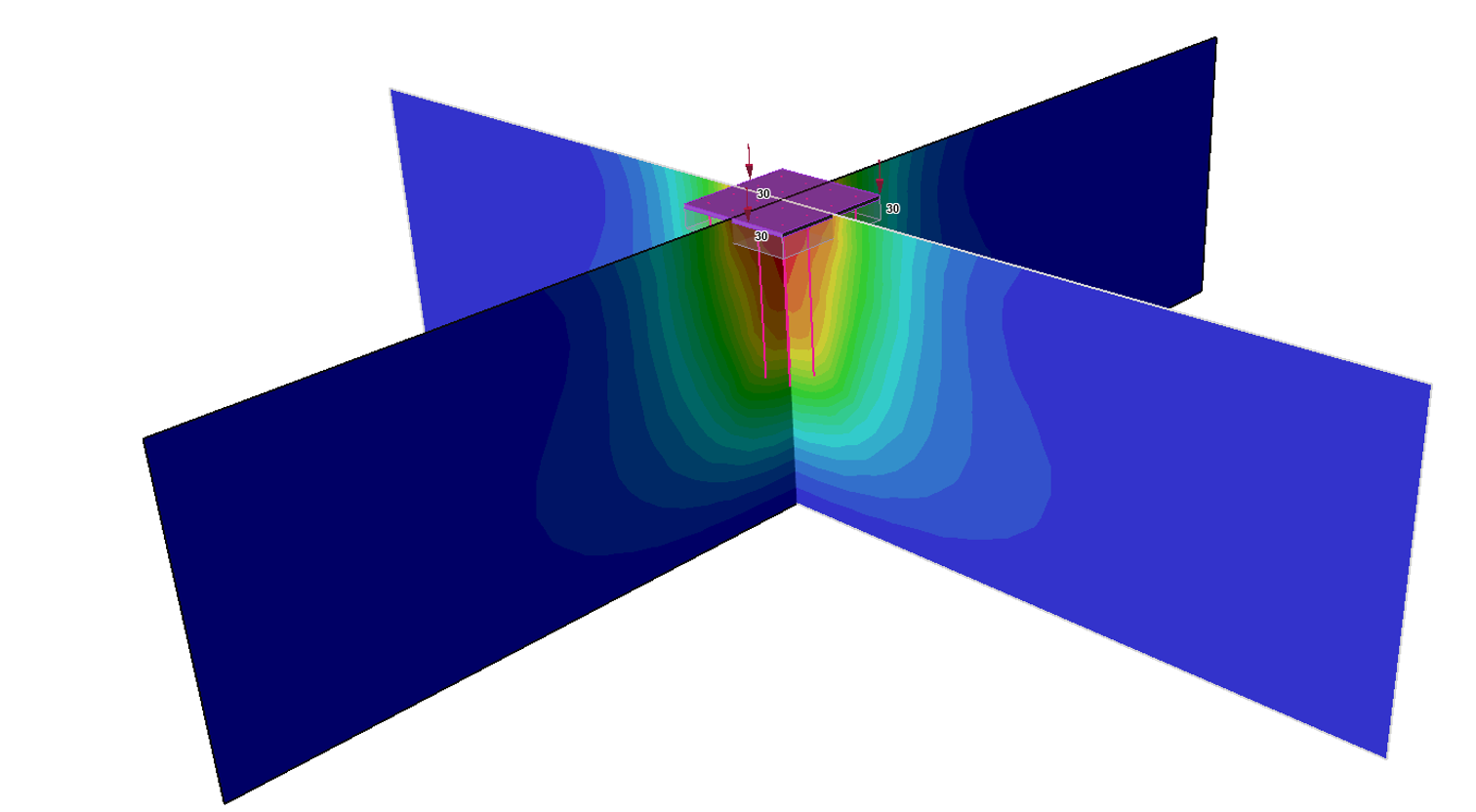
We can further improve the model by repeating the analysis in RS3 which can better capture 3D effects. Figure 7 presents the total displacement contours for the piled raft foundation design modelled in RS3 that shows similar deformations.
August 2020
Anisotropic Permeability: K1 Surface Option
As you know, when doing a seepage analysis in RS2, the soil permeability can either be defined as either isotropic or anisotropic. The permeability of the soil determines how the groundwater will drain and plays a critical part in performing a proper seepage analysis (as well as slope stability analysis). The pore water pressure distribution in your material affects directly affects the accuracy of the slope stability analysis and determining factor of safety.
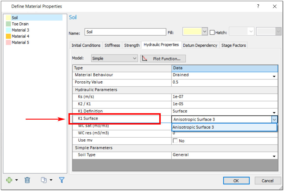
A new K1 Surface option was added that allows a user to assign the K1 line to an anisotropic surface. Previously users would enter a specific K1 angle. Now a drop-down option has been added to the Hydraulic Properties tab of the Define Materials dialog, which allows the user to select either the K1 Angle or K1 Surface option. If the user selects the K1 Surface option, they can select an anisotropic surface as the K1 line. Anisotropic surfaces can be added by selecting the Add Anisotropic Surface option in the Boundaries menu and applying it to your model with your mouse.
This quick and simple-to-use option can have a huge impact on the results of your analysis. As previously mentioned, getting a more accurate pore water pressure distribution means more accurate slope stability results and better-informed designs of slopes and supports. With this new option, users will have a much easier experience dealing with the real, practical problems of today, where materials are often not isotropic in their formation.
Other Ground Water Features
In addition to this soil permeability feature, two other exciting groundwater features have been added to the program.
A new option has been added to the Groundwater tab of your Project Setting for restraining excess pore pressure. If the checkbox for the Restrain excess pore pressure from undrained material option is selected, the excess pore pressure generated from the undrained material in your model will also follow the boundary conditions of the Finite Element Groundwater.
These mentioned Boundary Conditions now have additional functions as well. With joints, users can now select which side of a joint to apply the specific boundary conditions. This option becomes available when setting boundary conditions in a Steady State groundwater analysis. Specifically, if the Groundwater Method is selected as Steady State FEA or Transient FEA in Project Settings, then the groundwater (hydraulic) boundary conditions can be specified with the Set Boundary Conditions option in the Groundwater menu.
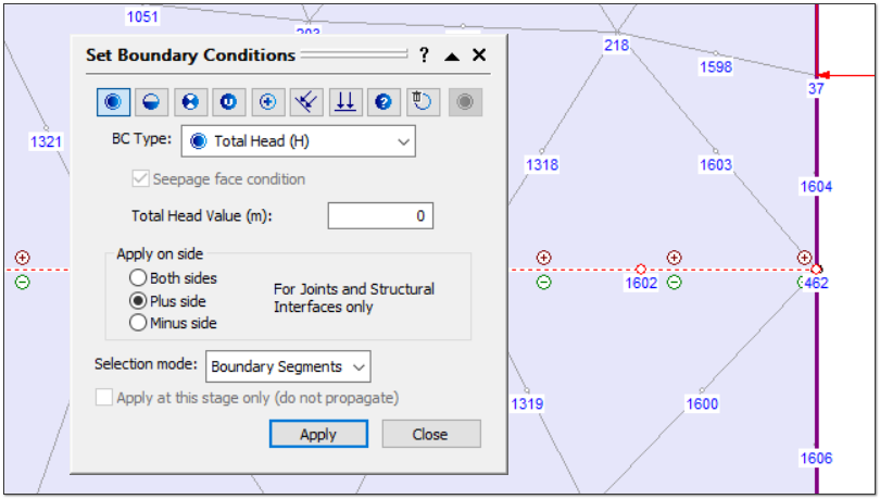
When a joint is selected, users are given the option to select a specific side of the joint indicated by a plus (+) or minus (-) symbol.
June 2020
Joint Strain-Softening
With exceptional analysis capabilities for both rock and soil, RS2 is your go-to finite element program for modeling and analyzing slopes, surface and underground excavations, groundwater seepage, consolidation, and much more. Its powerful, multi-core parallel processors allow you to solve complex finite element problems quickly and easily.
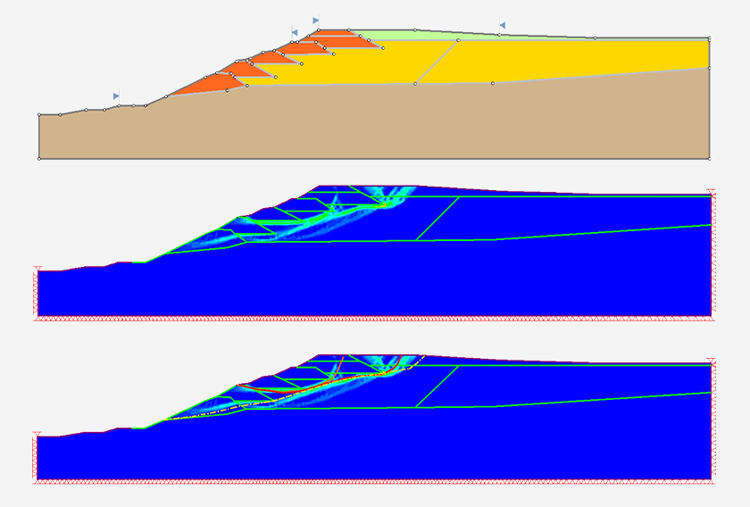
This month RS2 is adding a new joint strain-softening feature to its broad roaster of tools. As many know, modeling the behavior of soils at and after failure (as is necessary when modeling progressive failure of slopes) requires a relatively advanced constitutive relationship. The new displacement-softening and work-softening models have been developed to describe the sliding of geosynthetic interfaces, such as those in landfill liners.
March 2020
Dynamic Data Analysis in RS2
An accurate and efficient Dynamic Analysis of your model starts with the quality of your time history input data. That is why RS2 now features a new Dynamic Data Analysis option. When defining a Dynamic Load, you can now use the option to view, analyze, and filter load function input data before adding the load to your model.
Dynamic Data Analysis Dialog
At the core of the new option is the Dynamic Data Analysis dialog, which you can use to create a Dynamic Load Function. Once you create the function, you can assign it to one or more Dynamic Loads. To open the dialog, select Dynamic Data Analysis from the toolbar or the Dynamic menu.
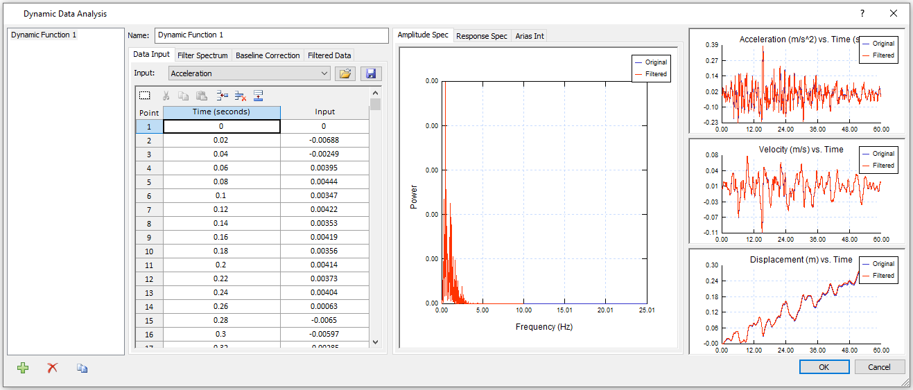
As shown in the figure above, the dialog is made up of three panels. The panel on the left displays the raw time history data and contains controls for various filtering options. The middle panel displays Amplitude Spectrum, Response Spectrum, and Arias Intensity graphs and the panel on the right displays Acceleration, Velocity, and Displacement vs. Time graphs.
Data Filtering
Several filtering options are available to make your Dynamic Analysis more efficient. As you apply these, the various graphs displayed in the dialog are dynamically updated to show both the original and filtered data for easy comparison.
One filtering option is the display of spectrum data for a given frequency range by entering a minimum and maximum in the Filter Spectrum tab. For example, if you observe in the Amplitude Spectrum graph that Amplitude is very minimal for frequencies larger than 10, you can set the maximum frequency to 10.
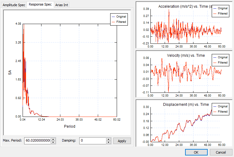
Another option is filtering data by maximum acceleration response to the load by adjusting the Maximum Period and Damping ratio at the bottom of the Response Spectrum graph.
Filtering all data by Dynamic Load Type by selecting Acceleration, Displacement, or Velocity from the Input dropdown is also an option in the left panel. Finally, you can additionally filter the Amplitude Spectrum by selecting a load type from the dropdown beneath the graph.
Baseline Correction
A part of these powerful filtering options is the ability to apply Baseline Correction in order to correct velocity and/or displacement drift. The option has two methods: Cut Off and Sinusoid. Once either Velocity or Displacement is corrected, new sets of Acceleration and Velocity or Acceleration and Displacement are calculated based on the corrected values and plotted on the graphs to compare with the original dataset.
Assigning a Dynamic Load Function to a Dynamic Load
Once a Dynamic Load Function is defined and saved, you can assign it to any Displacement, Acceleration, or Velocity Dynamic Load using the Define Dynamic Loads dialog. (Dynamic > Define Dynamic Loads). Clicking the X or Y Define button opens the Define Data dialog.
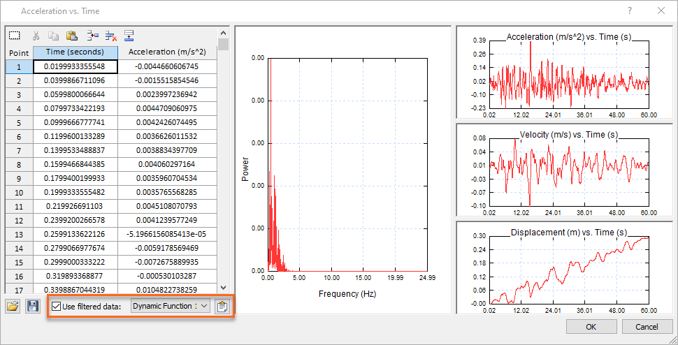
To apply the filtered data, simply select the Use Filtered Data checkbox at the bottom left of the dialog and then select the Dynamic Load Function from the dropdown to the right. To view and further filter the data, click the Filter Data button to the right of the dropdown. This opens the Dynamic Data Analysis dialog where you can analyze and filter the data as discussed above.
Dynamic Pore Pressure Analysis in RS2
RS2 now also has the Finn material model to enable more accurate computation of excess pore pressure generated by a seismic dynamic load. By applying the model to the analysis of a liquefiable material, you can better predict the increase of pore pressure and decrease of effective stress under the action of an external seismic load.
To enable this feature, select the Finn model as the material’s Strength Failure Criterion, then set the material’s Hydraulic Properties to Undrained. When Undrained is selected, you can manually input the Fluid Bulk Modulus to increase the numerical stability of your analysis.
Dynamic Boundary Conditions in RS2
Rounding out the roster of great new RS2 features is the addition of two new Dynamic Boundary Condition types: Hydro Mass and Nodal Mass. These options dramatically increase the power and flexibility of RS2’s Dynamic Analysis of dams and embankments.
The Hydro Mass option provides flexibility in RS2 to account for cases where the material is dry, but water is acting on its surroundings, such as a concrete dam. When selecting this boundary condition, you can manually enter pore pressure input as the height of the water in the reservoir as well as the base elevation of the reservoir.
The Nodal Mass option has bi-directional input and allows you to assign an additional mass to a node to simulate the dynamic load from an external force.
March 2020
Report Generator
This spring, Rocscience is excited to announce the introduction of the Report Generator, a dynamic new reporting tool coming to some of Rocscience's most powerful programs, including Slide2 & Slide3, RS2 & RS3, and EX3. Formerly called the Info Viewer, this new reporting tool lets you create sleek, professional-looking reports for your geotechnical project.
When you launch the Report Generator it will automatically create a report of your analysis, and package it with a customizable cover page, table of contents, headers and footers, and so much more.
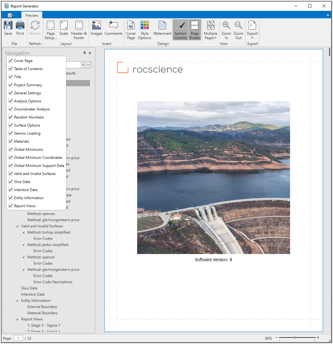
The Report Generator includes a navigation bar that lets you quickly navigate and search the report. Just click on the document map to view sections of the report or use the search bar to look for specific content. Included in the report is a table of contents that is automatically created and adjusted as you add and remove sections from your analysis.
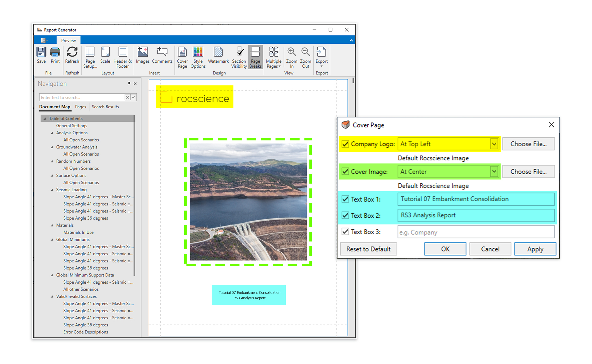
A sleek, editable cover page is automatically created for your report and can be customized with your own images, company logo, and more. Use the controls to easily adjust the layout and select what sections to include. Once you’re happy with the look of your cover page, you can save time by saving these customizations for use on future projects.
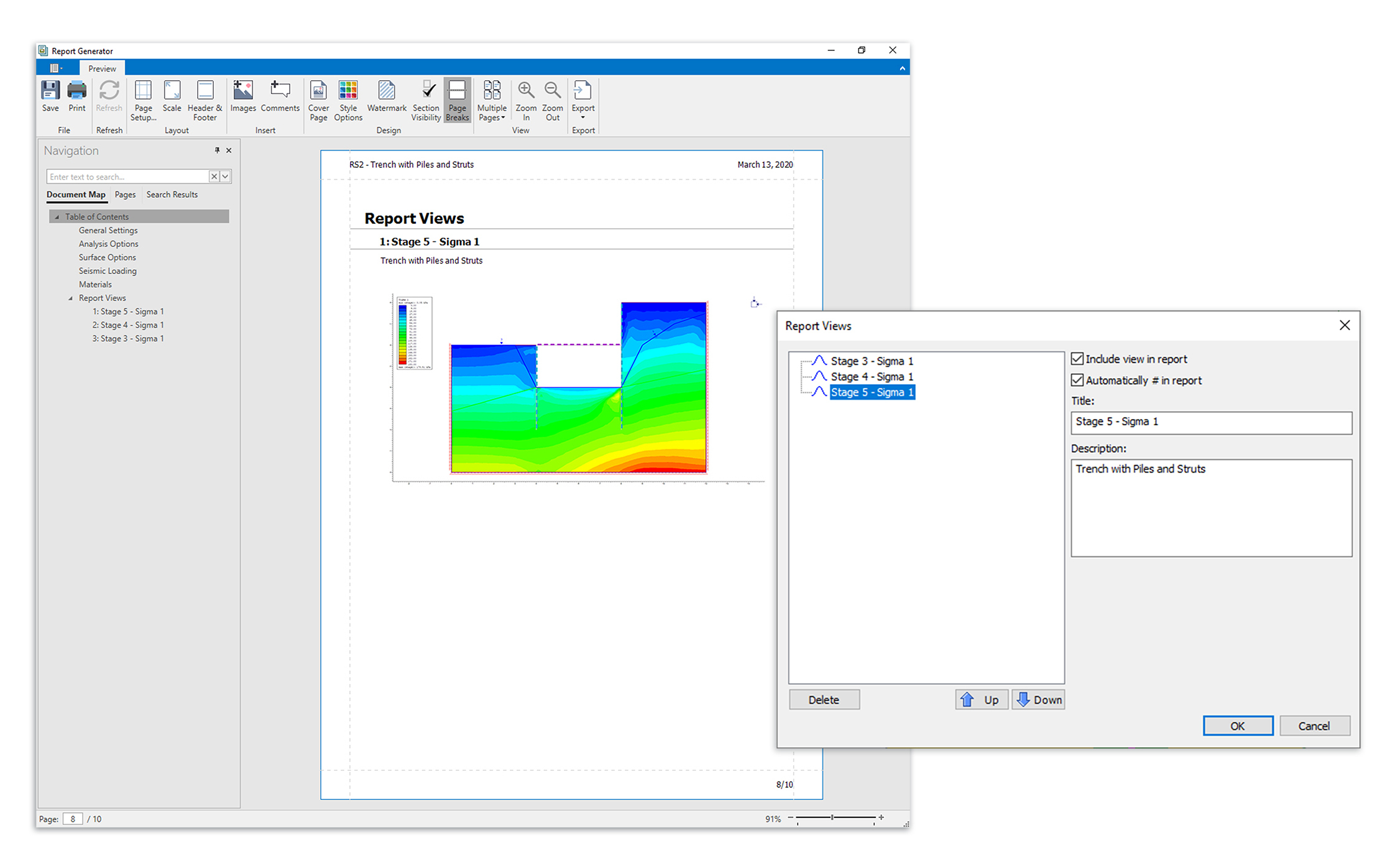
With the Report Generator, you can edit more than just the look of your report though. You can also add content of your own! Use the Add Images or Add Comments buttons to add text and images to any section of the report. If you want to add snapshots of the computed model, you can do that as well from the Interpret window of your Rocscience program. The tool lets you add multiples views of your model, add titles and descriptions, and even arrange the order of the views. The views of the model will then be added to the end of your report.
Once you’re done customizing your report, you can easily print or export the file.
December 2018
Wick Drains and Vacuum Consolidation
One of the new features in RS2 2019 is the ability to model wick drain installations when analyzing time-dependent soil consolidation with transient groundwater seepage analysis. The feature includes the optional use of vacuum consolidation, a soil improvement method often used in conjunction with wick drain installation.
Wick drains are installed in soft soils to accelerate the rate of consolidation. The drains are typically made up of a plastic strip with drainage patterns wrapped in a geotextile filter that prevents soil particles from entering the channels and clogging the drain. Wick drains shorten the drainage path of pore water, allowing soil consolidation to occur in a matter of weeks rather than years.
The vacuum consolidation method is a construction improvement technique for consolidating and stabilizing soft clayey soil. It is often used in conjunction with wick drain installations and works by applying vacuum suction to a soil mass to reduce pore water pressure.
Learn RS2
Explore the RS2 user guide for in-depth instructions on how to use the program and visit our library of learning resources, including case studies, past webinars, and articles, designed to expand your geotechnical knowledge and help you get the most out of your analysis.