Integrating Machine Learning and RS3: Modernizing Back-Analysis for Slope Stability

In open-pit mining, failure can be remarkably legible. Modern mapping technologies let engineers reconstruct the geometry of rock joints and fault surfaces with incredible precision — the dip, the strike, the intersections that define how a wedge might release.

But there is a hidden variable that remains stubbornly out of reach: the actual shear strength of those structures. Friction angle and cohesion cannot be read from a borehole log or measured reliably in a laboratory. They must be inferred from events that have already happened, from slopes that have already moved. This process, known as back-analysis, is where the precision of modern mapping runs headlong into the ambiguity of geomechanical reality.

Traditionally, finding these hidden values required running massive 3D simulations that could take days to solve. To get it right, engineers often had to manually test hundreds of scenarios, a process that is not only labour-intensive but often impractical in fast-moving mining environments.

This case study, based on the research of McQuillan, Mitelman, and Elmo (2023), presents a different approach. By coupling machine learning (ML) with RS3, Rocscience’s 3D finite-element software, the workflow transforms back-analysis from selective iteration into a structured exploration of the full parameter space, producing not just a plausible calibration, but a defensible one.

Project Overview

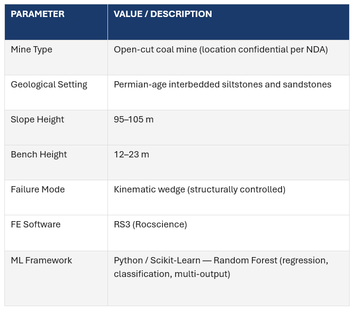
Geological and Structural Context

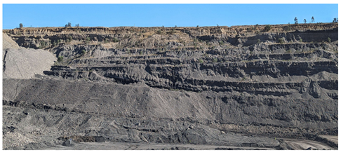
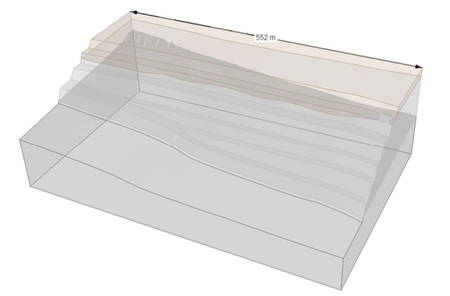
In this case, the slope is sourced from an open-cut coal mine as shown in Figure 1. The slope intersects Permian-age sedimentary strata of interbedded siltstones and sandstones, with bedding thicknesses ranging from 1 to 5 m. The upper bench comprises weathered Permian material overlying fresh Permian units, grouped into a single rock mass domain for modelling purposes.

Stability is governed by the intersection of three sub-vertical fault systems and a basal sub-horizontal shear plane, designated H15 (top of coal). Together, these four structures define a classic kinematic wedge: the faults form the lateral release surfaces; H15 provides the basal sliding plane.

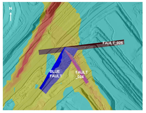
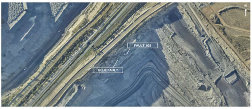
While the wedge geometry is well-constrained, the frictional resistance of the sub-vertical faults cannot be measured directly. This is the central calibration challenge the workflow addresses.

RS3 as the Engine of Structured Data Generation

In this workflow, RS3 is used not merely as a solver, but as a systematic generator of simulation data. Python-based scripting interfaced with RS3's input file to automate model duplication, parameter variation, batch execution, and results extraction.

Model Construction

The slope geometry was reconstructed in RS3 using high-resolution aerial imagery and topographic survey data. Rather than modelling the full open-pit extent, a representative 3D section capturing the wedge failure zone was simulated as shown in Figure 3.

Two deliberate simplifications were applied:

• Only a representative section of the pit was modelled.
• Intact rock materials were treated as elastic, reducing computational demand and improving convergence efficiency.

Due to the inherent computational demands of 3D SSR analysis, combined with the scale and resolution of the model, each simulation can take several hours to solve. This makes traditional, large-scale parametric back-analysis workflows difficult to implement in practice; thereby underscoring the importance of an automated calibration workflow.

Joint Representation and Parameter Space

The three controlling faults and the H15 basal shear were modelled as explicit zero-thickness joint elements. Eight input variables representing joint properties across two joint sets were derived from four parameters – friction angle (φ), cohesion (c), normal stiffness (Kn), and shear-to-normal stiffness ratio (Ks/Kn) – applied independently to each of the two joint sets.

A uniform distribution was used to randomize the joint parameters ensuring full coverage of the parameters, including conditions near failure, where ML models need representative data most. Uniform sampling ensures balanced representation across the parameter, improving machine learning training stability and reducing bias toward clustered values.

Machine Learning as a Calibration Tool

Each RS3 simulation produced two critical data points: maximum displacement (how much the rock moved) and model convergence (whether the physics of the model held together).

In numerical rock mechanics, non-convergence is not simply a computational inconvenience; it is a meaningful signal. When a model fails to converge, the physics of the system have broken down, and the displacement values it generates become numerically unstable. Recognizing this, the team used convergence as a binary classifier, separating simulations that represented stable behaviour from those that indicated collapse.

To process this, Random Forest (RF) algorithms were trained using three approaches: a regression model predicting maximum displacement, a classification model distinguishing stable from unstable behaviour, and a multi-output model combining both objectives. The goal here wasn't just to predict a number, but to perform a sensitivity audit; pinpointing exactly which geological inputs were driving the failure and which were just background noise.

The most important breakthrough was finding was the efficiency of the workflow. Rather than running hundreds of time-consuming simulations, the team monitored the ML model’s performance in real-time. the team stopped. That point arrived after just 30 simulations, a striking result for a problem with an eight-dimensional parameter space and models requiring several hours each to solve. This proved that ML-assisted back-analysis is a practical, feasible tool for complex 3D workflows where every hour of computation counts. 

Results: When the Problem Collapses

ML Model Performance

All three Random Forest model types achieved acceptable predictive performance across the 30-simulation dataset. The classification model was exact, distinguishing stable from unstable models without a single misclassification, with 100% accuracy. Displacement predictions showed errors in the range of 1.5 to 3 metres, not because the model was poorly trained, but because near-failure numerical behaviour is genuinely noisy. As a slope approaches total collapse, displacement values reflect a system at its limits, not a smoothly predictable physical process. Some variance here is expected, and its presence is informative.

Feature Importance: The Problem Resolves to One Variable

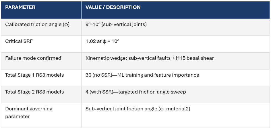
The most consequential outcome of this analysis was not predictive accuracy. It was what the models revealed about the structure of the problem itself. Feature importance analysis, conducted across all three Random Forest model types, consistently identified a single dominant variable: the friction angle of the sub-vertical joints. Cohesion, stiffness parameters, and basal shear properties all registered as negligible within the defined parameter ranges and modelling assumptions. 
 

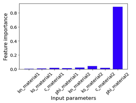
This finding is geomechanically consistent. The sub-vertical faults define the lateral kinematic release surfaces of the wedge, and their frictional resistance determines whether the wedge mobilizes. The machine learning models, trained only on simulation inputs and outputs, converged on the same conclusion that structural geology would suggest, but they did so without assuming it in advance.

The practical implication is decisive: an eight-parameter calibration problem collapses to a single governing variable.

Targeted SSR Calibration

With the parameter space resolved, a targeted sweep of sub-vertical joint friction angle was conducted using RS3's shear strength reduction (SSR) capability, ranging from 7° to 10°. All non-dominant parameters were fixed at their mean values, directing the remaining computational effort exclusively toward the variable that mattered.

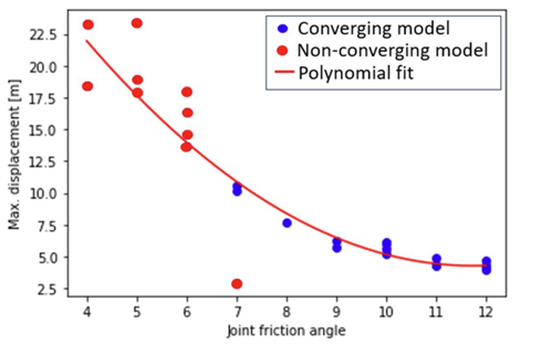
The results were unambiguous. As friction angle fell below approximately 8°, displacement increased non-linearly, and the model at 7° ceased to converge, marking the numerical threshold of instability. The model with φ = 10° produced a strength reduction factor of 1.02, consistent with the meta-stable conditions at observed failure. The calibrated friction angle is therefore: 9°–10°.
 

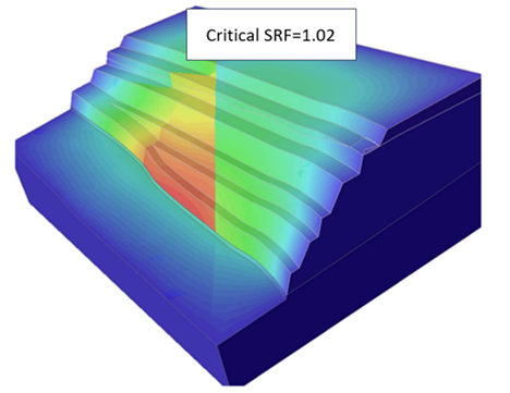
Displacement patterns aligned with the observed wedge geometry, confirming both the failure mechanism and the calibration.

Key Results Summary

What This Changes for Engineering Practice

The efficiency gains are real, but they point to something more fundamental: a change in how the problem is approached from the outset.

• From selective iteration to full coverage: the parameter space is explored systematically, not by intuition.
• From uncertainty to governing variables: feature importance isolates what actually controls failure, before any targeted calibration begins.
• From model execution to model interrogation: RS3 becomes a tool for extracting structural insight, not just generating results.

Several caveats deserve explicit acknowledgement. While the methodology is transferable, the calibrated values are not. Results remain case-specific and dependent on geometry, parameter ranges, and modelling assumptions. The authors also caution against over-automation: near-failure numerical behaviour requires engineering judgment to interpret, and the workflow is designed to support that judgment.

Conclusion: A Shift in How Back-Analysis Is Done

The detachment of a rock wedge is simultaneously a loss of stability and a gain of information. What this case study demonstrates is not simply faster calibration; it is a more rigorous approach to uncertainty in three-dimensional numerical modelling.

By using RS3 to generate structured, machine-interpretable simulation data, machine learning to identify what governs the system, and SSR analysis targeted at the variable that actually matters, the workflow produces a calibrated result that is traceable and defensible in ways that manual iteration rarely achieves.

The calibrated friction angle of 9°–10°, derived from 34 RS3 simulations, provides a foundation for forward-looking stability assessment at this mine. More broadly, it offers a template: back-analysis conducted not as a search for any answer that fits, but as a systematic narrowing toward the answer that the physics demands.