Introduction

Seepage analysis plays a pivotal role in various engineering applications, such as ensuring the safety, stability, and sustainability of slopes, infrastructure, and natural ecosystems. Accurate analysis results can help prevent potential seepage-induced disasters such as dam failures and landslides. As such, the usage of a seepage analysis software that can reliably predict groundwater flow patterns in the most complex situations is paramount. However, often users will first verify the results from a software with analytical solutions before accounting for more complicated conditions.

In this article, two case studies are examined in RS2 to highlight the effects of anisotropic conditions and saturated-unsaturated regimes on seepage analysis compared to ones that use a traditional approach.

Case I: Effect of Anisotropy on Flow Net Shape

Flow nets are essential tools for analyzing the movement of groundwater through soil structures, as they provide insight to seepage patterns and aid in design and stability assessment. A flow net consists of 2 families of lines: streamlines which represent the direction of water particle flow, and equipotential lines which represent lines of constant total head.

In soils that exhibit isotropic permeability, streamlines are always perpendicular to equipotential lines for every point in the flow net. However, in most engineering applications soil permeability is anisotropic due to factors such as compaction and loading, which often results in the horizontal permeability being much greater than the vertical. In these cases, streamlines are no longer orthogonal to the equipotential lines, resulting in a skewed mesh. For the case Kx > Ky, the flow net will have a stretched appearance.

Model Geometry

In RS2, we can compare the flow nets for isotropic and anisotropic soils by adjusting the ratio for the horizontal and vertical permeabilities in the hydraulic properties tab.

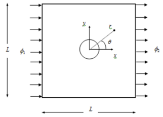
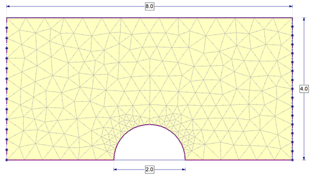
In this study we will be examining a problem which consists of uniform fluid flow around a 1m radius cylinder as shown in Figure 1. Due to its symmetry about the x-axis, only the upper half of the domain is modelled in RS2. The hydraulic boundary condition is set to total head of 1m on the left and 0m on the right. The dimensions of the tunnel are also shown in Figure 2.

We can define the ratio for the horizontal and vertical permeability with the K2 / K1 parameter. K2 is the vertical permeability while K1 is the horizontal. In Table 1, the ratio is set to 0.1, meaning the horizontal permeability is greater than the vertical by a factor of 10.

Table 1: Hydraulic properties K2=0.1K1

Parameter	Value
Model	User Defined
Material Behavior	Drained
K2/K1	0.1
K1 Definition	Angle
K1 Angle (degrees)	0
Permeability and Water Content
Permeability - 0 kPa Suction (m/s)	1e-5
Permeability - 100 kPa Suction (m/s)	1e-5

Results

In this analysis, permeability ratios of 1, 0.5, 0.1, and 0.01 were used. Flow nets can be constructed in the interpreter by turning the contour mode to “Filled (with lines)” to show equipotential lines and using the “Add Multiple Flow Lines” tool to show equidistant streamlines. The results are shown below.

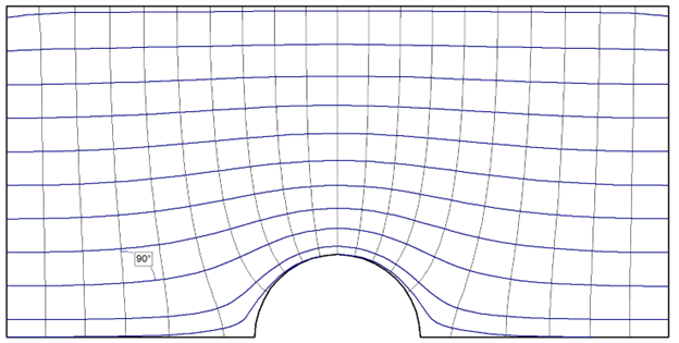
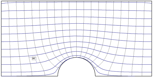
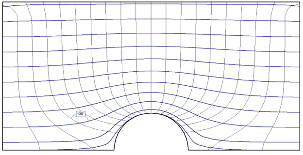
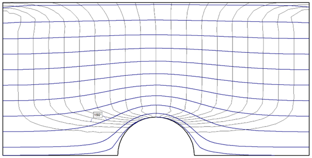
From Figure 3 to Figure 6 above, we can notice that as the K2 / K1 ratio decreases, or as horizontal permeability becomes even greater than the vertical, the skew of the flow lines to the equipotential lines becomes more pronounced, especially around the tunnel area. For reference, angle markings have been included in each figure to illustrate how the line intersection at a particular point increases from 90 degrees for isotropic soil to 150 degrees for the most extreme anisotropic case.

Case II: Modelling Saturated vs. Saturated-Unsaturated Flow in RS2

Seepage plays a critical role in the failure of dams because of its potential to cause slope instability, erosion, and saturation-induced strength reduction. As such, accurate analysis of flow through a dam is important for determining its safety.

Traditional models for groundwater seepage consider flow only in the saturated zone, such as the unconfined flow net technique proposed by Casagrande (1937). This technique treats the upper surface of the flow net (the phreatic surface) as the upper boundary on seepage and ignores all flow occurring in the unsaturated region. However, it is well known that flow also exists in the unsaturated zone, and the use of traditional methods in these situations typically overestimates the elevation of the water table.

Model Geometry

We can model both flow methods in RS2 by setting different hydraulic models in the hydraulic properties tab.

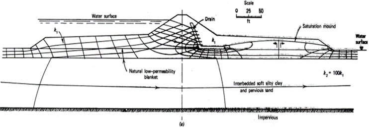
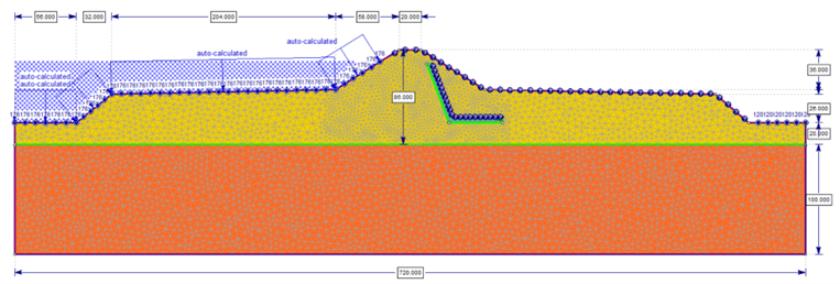
In this study we will be examining an earth dam with a chimney drain example from Cedergren (1989) as shown in Figure 7, which uses the traditional saturated flow method. The dam consists of two soil layers, with the bottom layer having permeability 100 times that of the top layer. Both soil layers are assumed to be anisotropic with the horizontal permeability nine times the vertical. A total head of 176m is applied to the submerged section of the left side of the dam and 120m is applied to the water surface at the right side of the dam as shown in Figure 8.

2 models were created, one using the saturated-unsaturated flow method and the other using the saturated flow method.

Hydraulic models included in RS2 automatically account for the unsaturated flow above the phreatic surface. For this particular model, we use the “Simple” model for all the material. In the hydraulic properties tab, set the horizontal permeability Ks to 1000 ft/s for the earth dam, 1e6 ft/s for the drain, and 1e5 ft/s for the foundation material. For all materials set the K2/K1 ratio to 0.111111 to simulate anisotropy. Leave all other properties as their default values. Hydraulic properties are shown in Table 2 below.

Table 2: Hydraulic properties – saturated-unsaturated model

Parameter	Earth Dam	Drain	Foundation
Model		Simple
Material Behaviour		Drained
K2/K1		0.111111
K1 Definition		Angle
K1 Angle (degrees)		0
Ks (ft/s)	1000	1e+6	100000

In order to model the traditional approach where no flow is allowed in the unsaturated zone, we can use the “User defined” hydraulic model to specify a permeability function for each material. Click “Define” to input a table of matric suction vs. permeability data in the permeability and water content dialog. For 0 matric suction (for regions below the phreatic surface), the permeability values are 1000, 1e+6, and 1e+5 for earth dam, drain, and foundation materials respectively. Then for 0.001 matric suction, the permeability is set to the smallest possible value for all materials, which in RS2 is 1e-12. This essentially reduces all flow above the phreatic surface to zero, which is required for the traditional saturated flow method. Hydraulic properties are shown in Table 3 below.

Table 3: Hydraulic properties – traditional model

Parameter	Earth Dam	Drain	Foundation
Model		User Defined
Material Behaviour		Drained
K2/K1		0.111111
K1 Definition		Angle
K1 Angle (degrees)		0
Permeability and Water Content
Permeability – 0 psf Suction (ft/s)	1000	1e+6	100000
Permeability – 0.001 psf Suction (ft/s)		1e-12

Results

The results of both models are shown below, with Figure 9 using the traditional saturated flow method and Figure 10 using the saturated-unsaturated method. In the saturated flow case, the phreatic surface intersects the drain near the top of the vertical section, matching the flow net from the example in Cedergren (1989). For the saturated-unsaturated case, the phreatic surface intersects lower at the horizontal section of the drain.

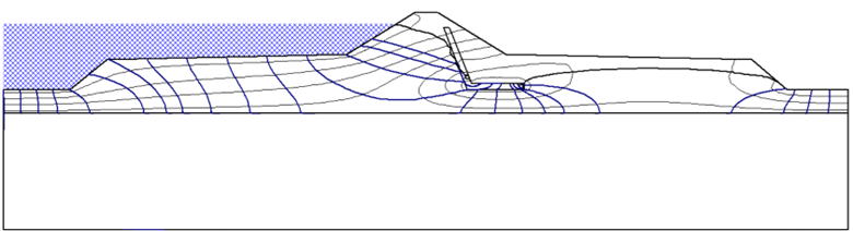
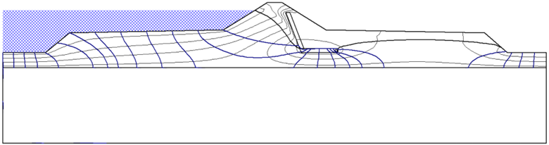
The difference in phreatic surface elevation is due to conservation of mass flow. In the saturated-unsaturated case, seepage occurs above and below the phreatic surface. In the pure saturated flow case, the seepage occurring above the phreatic surface is ignored. By conservation of mass that flow must therefore occur below the phreatic surface, which increases the elevation of the water table.

Conclusion

Modern software tools have significantly advanced the capability to carry out realistic seepage analysis. These software solutions can also yield results comparable to those obtained through traditional methods, when employing the same assumptions – for instance, the omission of flow within the unsaturated zone. This technological evolution not only enhances the precision of seepage analysis but also simplifies the integration of established techniques into workflows, contributing to more efficient and accurate assessments of seepage-related problems in various engineering and environmental applications.

References

Casagrande, A. (1937). Seepage through dams. New England Water Works. 51(2), pp. 295-336.

Cedergren, H.R. (1989). Seepage, drainage, and flow nets. Wiley-InterScience, John Wiley & Sons, New York.

More from Rocscience